load("C:/BLOG/Workspaces/NIT Tutorial/NIT_ws12.RData")
library(tidymodels)
library(caret)Splitting the data before the calibration.
In this post we are going to use the package Caret to develop PLS models for protein, fat and moisture, but first we have to split the data in two sets, one for training and other for testing. Now we load the libraries we need, and the workspace from the previous post.
We did use Caret to split the tecator data in the post NIT_tutorial_5, so we repeat the process again with our last dataframe (from the previous post “tecator2”):
set.seed(1234)
tecator2_split_prot <- initial_split(tecator2, prop = 3/4, strata = Protein)
tecator2_split_fat <- initial_split(tecator2, prop = 3/4, strata = Fat)
tecator2_split_moi <- initial_split(tecator2, prop = 3/4, strata = Moisture)

tec2_prot_train <- training(tecator2_split_prot)
tec2_prot_test <- testing(tecator2_split_prot)

tec2_fat_train <- training(tecator2_split_fat)
tec2_fat_test <- testing(tecator2_split_fat)

tec2_moi_train <- training(tecator2_split_moi)
tec2_moi_test <- testing(tecator2_split_moi)
We have done this in a random way, so we expect that some of the mahalanobis distance outliers samples have gone to the training set and the remaining to the test set. Now, we can start to develop the regressions with the training set, and the validation with the test set, using the Caret package with the “pls” algorithm. We will use the cross validation (10 folds), to select the number of terms.
Model and validation performance for Protein
set.seed(1234)
ctrl <- trainControl(method = "cv", number = 10)
tec2_pls_model_prot <- train(y = tec2_prot_train$Protein,
  x = tec2_prot_train$snvdt2der2_spec,
  method = "pls",
  trControl = ctrl)


tec2_pls_model_prot
Partial Least Squares
160 samples
100 predictors
No pre-processing
Resampling: Cross-Validated (10 fold)
Summary of sample sizes: 144, 144, 144, 144, 144, 143, ...
Resampling results across tuning parameters:
ncomp RMSE Rsquared MAE
1 1.451693 0.7398494 1.0940694
2 1.342024 0.7854652 1.0083106
3 1.301409 0.8228018 0.9822213
RMSE was used to select the optimal model using the smallest value.
The final value used for the model was ncomp = 3.now we can see how the model performs with the test set, and create a table with the “SampleID
pls_preds <- predict(tec2_pls_model_prot, tec2_prot_test$snvdt2der2_spec)
test_prot_preds <- bind_cols(tec2_prot_test$SampleID ,tec2_prot_test$Protein, pls_preds, tec2_prot_test$outlier)
colnames(test_prot_preds) <- c("SampleID", "Prot_lab", "Prot_pred", "Outlier")
an XY plot (laboratory vs. predicted values) can gives an idea of the performance of the validation test:
test_prot_preds %>%
  ggplot(aes(x = Prot_lab, y = Prot_pred, colour = Outlier)) +
  geom_point(size = 3) +
  geom_abline() +
  scale_color_manual(values = c("no outlier" = "green",
                                "Warning outlier" = "orange",
                                "Action outlier" ="red"))
Model and validation performance for Fat
set.seed(1234)
ctrl <- trainControl(method = "cv", number = 10)
tec2_pls_model_fat <- train(y = tec2_fat_train$Fat,
  x = tec2_fat_train$snvdt2der2_spec,
  method = "pls",
  trControl = ctrl)


tec2_pls_model_fat
Partial Least Squares
160 samples
100 predictors
No pre-processing
Resampling: Cross-Validated (10 fold)
Summary of sample sizes: 144, 145, 143, 144, 144, 144, ...
Resampling results across tuning parameters:
ncomp RMSE Rsquared MAE
1 2.339072 0.9731581 1.832527
2 2.276391 0.9762236 1.757150
3 2.215674 0.9782784 1.744476
RMSE was used to select the optimal model using the smallest value.
The final value used for the model was ncomp = 3.now we can see how the model performs with the test set, and create a table with the “SampleID
pls_preds_fat <- predict(tec2_pls_model_fat, tec2_fat_test$snvdt2der2_spec)
test_fat_preds <- bind_cols(tec2_fat_test$SampleID ,tec2_fat_test$Fat, pls_preds_fat, tec2_fat_test$outlier)
colnames(test_fat_preds) <- c("SampleID", "Fat_lab", "Fat_pred", "Outlier")
test_fat_preds %>%
ggplot(aes(x = Fat_lab, y = Fat_pred, colour = Outlier)) +
geom_point(size = 3) +
geom_abline() +
scale_color_manual(values = c("no outlier" = "green",
"Warning outlier" = "orange",
"Action outlier" ="red"))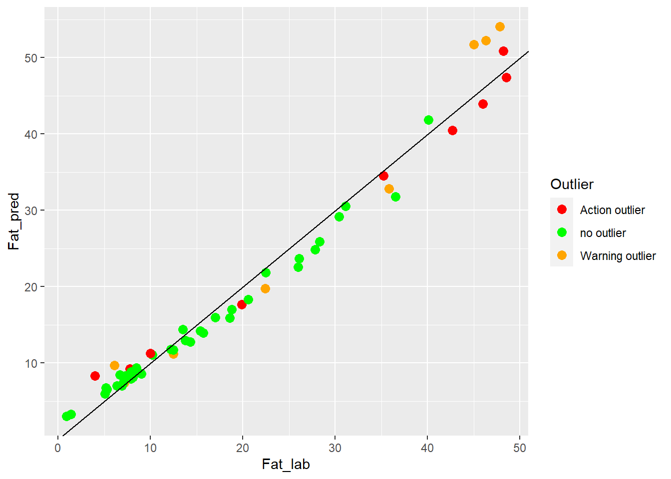
Model and validation performance for Moisture
set.seed(1234)
ctrl <- trainControl(method = "cv", number = 10)
tec2_pls_model_moi <- train(y = tec2_fat_train$Moisture,
  x = tec2_fat_train$snvdt2der2_spec,
  method = "pls",
  trControl = ctrl)


tec2_pls_model_moi
Partial Least Squares
160 samples
100 predictors
No pre-processing
Resampling: Cross-Validated (10 fold)
Summary of sample sizes: 144, 144, 143, 144, 144, 144, ...
Resampling results across tuning parameters:
ncomp RMSE Rsquared MAE
1 2.080841 0.9583109 1.641792
2 2.031741 0.9600832 1.593240
3 2.014572 0.9612094 1.566407
RMSE was used to select the optimal model using the smallest value.
The final value used for the model was ncomp = 3.now we can see how the model performs with the test set, and create a table with the “SampleID
pls_preds_moi <- predict(tec2_pls_model_moi, tec2_moi_test$snvdt2der2_spec)
test_moi_preds <- bind_cols(tec2_moi_test$SampleID ,tec2_moi_test$Moisture, pls_preds_moi, tec2_moi_test$outlier)
colnames(test_moi_preds) <- c("SampleID", "Moi_lab", "Moi_pred", "Outlier")
test_moi_preds %>%
ggplot(aes(x = Moi_lab, y = Moi_pred, colour = Outlier)) +
geom_point(size = 3) +
geom_abline() +
scale_color_manual(values = c("no outlier" = "green",
"Warning outlier" = "orange",
"Action outlier" ="red"))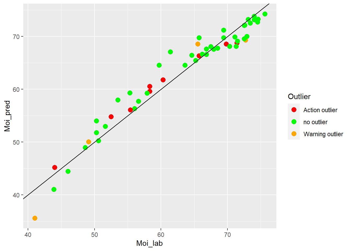
Now I save the workspace to continue in the next post
save.image("C:/BLOG/Workspaces/NIT Tutorial/NIT_ws13.RData")Table of results
| Parameter | N training | N test | Terms | C.V. error (SECV) | Test Pred. error (SEV) |
|---|---|---|---|---|---|
| Protein | 160 | 55 | 3 | 1.30 | 1.49 |
| Fat | 160 | 55 | 3 | 2.22 | 2.34 |
| Moisture | 160 | 56 | 3 | 2.01 | 2.25 |
Conclussions
With all the plots above we can ask ourselves several questions in order to find the better performance we can get from the data.
Can we force the model to use more terms , (few for the complexity of the data) , does this option improves the results on the test set?
Can we use another model algorithm (different to “pls”) to improve the results?.
- do we have enough samples for those algorithms?
Does the “non MD outliers” samples predict better than the “warning” or “action” MD outliers?
Do we see non linearities in the plots?
- How we can manages these non linearities?
- Maybe adding more terms to the PLS model we improve the linearity.
Comment any other conclusions you have.