load("C:/BLOG/Workspaces/NIT Tutorial/NIT_ws13.RData")
library(tidyverse)
library(caret)Continuing from the previous post, we will try in this one to improve our models adding if necessary more terms, but taking care not to overfit them. Let´s load the previous workspace.
New model for Protein
Now we develop (like in the first post) the protein model, and select a maximum of 20 “pls” terms:
set.seed(1234)
tec2_pls_model2_prot <- train(y = tec2_prot_train$Protein,
  x = tec2_prot_train$snvdt2der2_spec,
  method = "pls",
  tuneLength = 20,
  trControl = ctrl)

tec2_pls_model2_prot
Partial Least Squares
160 samples
100 predictors
No pre-processing
Resampling: Cross-Validated (10 fold)
Summary of sample sizes: 144, 144, 144, 144, 144, 143, ...
Resampling results across tuning parameters:
ncomp RMSE Rsquared MAE
1 1.4516929 0.7398494 1.0940694
2 1.3420243 0.7854652 1.0083106
3 1.3014092 0.8228018 0.9822213
4 1.1259765 0.8674607 0.8603669
5 1.0438039 0.9015276 0.7756167
6 0.9546769 0.9115595 0.7173969
7 0.7224697 0.9428984 0.5395207
8 0.6293469 0.9560991 0.4905239
9 0.5873218 0.9625907 0.4489137
10 0.5725280 0.9643334 0.4371128
11 0.5781189 0.9634284 0.4407352
12 0.6032003 0.9596191 0.4488933
13 0.5921560 0.9605140 0.4494456
14 0.5722990 0.9640706 0.4420770
15 0.5637927 0.9651988 0.4421589
16 0.5708793 0.9644509 0.4409289
17 0.5961376 0.9619309 0.4483742
18 0.6122767 0.9601094 0.4530714
19 0.6219969 0.9568690 0.4594357
20 0.6111615 0.9612657 0.4668470
RMSE was used to select the optimal model using the smallest value.
The final value used for the model was ncomp = 15.The reason to select 15 is simple, the RMSE for cross validation has its minimum at 15 terms and after starts to increase (Take into account if other seed is selected other number of terms probably would be selected).
Now, we have a new model with 15 terms indeed 3, but how this affect to the predictions of the test set:
pls_preds2 <- predict(tec2_pls_model2_prot, tec2_prot_test$snvdt2der2_spec)
test_prot_preds2 <- bind_cols(tec2_prot_test$SampleID ,tec2_prot_test$Protein, pls_preds2, tec2_prot_test$outlier)
colnames(test_prot_preds2) <- c("SampleID", "Prot_lab", "Prot_pred", "Outlier")
let´s see if the XY plot (laboratory vs. predicted values) can gives an idea of the performance of the validation test:
test_prot_preds2 %>%
  ggplot(aes(x = Prot_lab, y = Prot_pred, colour = Outlier)) +
  geom_point(size = 3) +
  geom_abline() +
  scale_color_manual(values = c("no outlier" = "green",
                                "Warning outlier" = "orange",
                                "Action outlier" ="red"))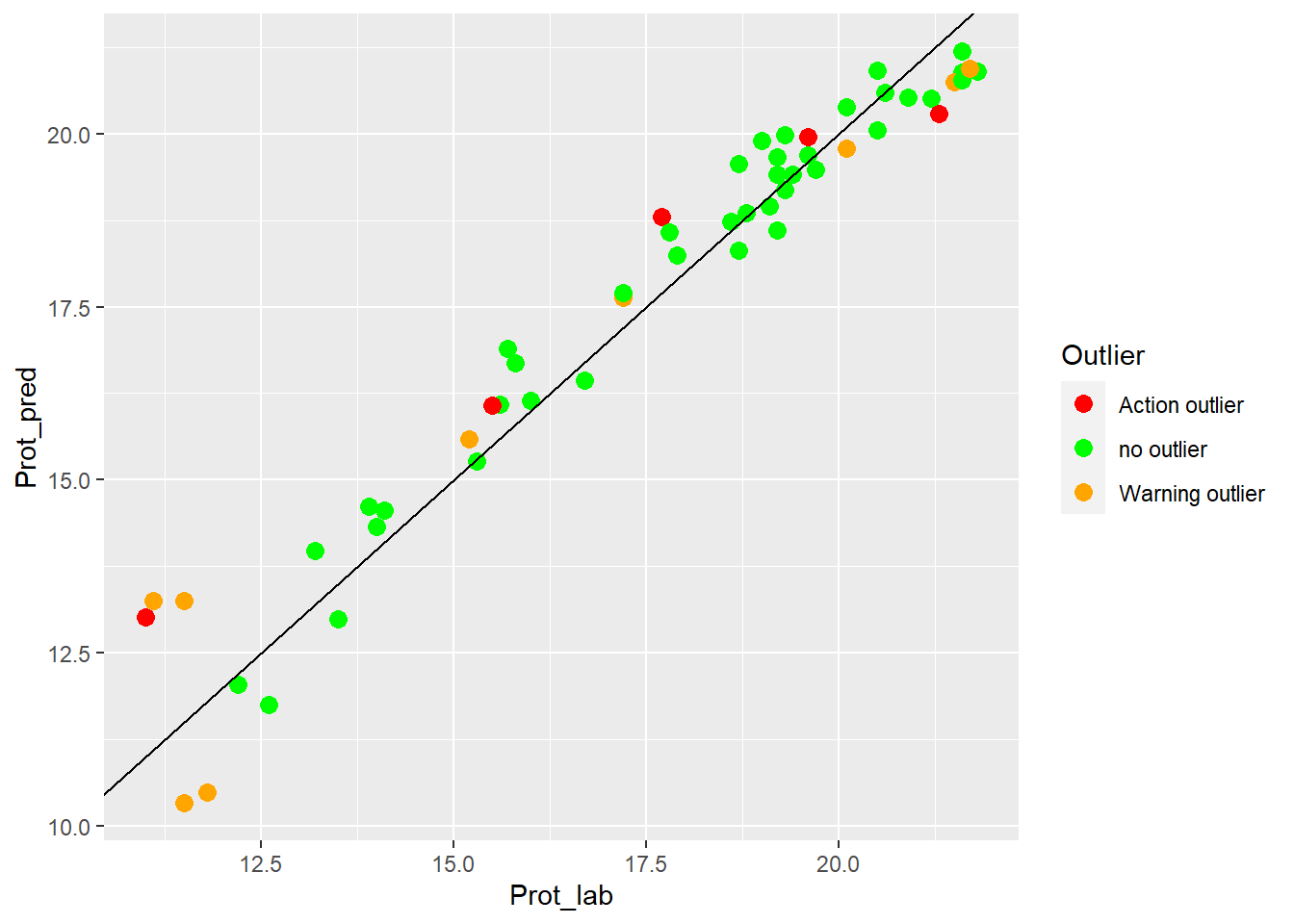
Clearly we can see the improvement in fit of the dots vs. the line.
Now we can develop the regressions for fat and moisture:
New model for Fat
set.seed(1234)
tec2_pls_model2_fat <- train(y = tec2_moi_train$Fat,
  x = tec2_moi_train$snvdt2der2_spec,
  method = "pls",
  tuneLength = 20,
  trControl = ctrl)

tec2_pls_model2_fat
Partial Least Squares
159 samples
100 predictors
No pre-processing
Resampling: Cross-Validated (10 fold)
Summary of sample sizes: 143, 144, 143, 143, 143, 143, ...
Resampling results across tuning parameters:
ncomp RMSE Rsquared MAE
1 2.336132 0.9719221 1.876665
2 2.302221 0.9732855 1.865222
3 2.275123 0.9743372 1.808143
4 2.201834 0.9767875 1.740885
5 2.171390 0.9782392 1.686537
6 2.124222 0.9788118 1.662976
7 2.065867 0.9786525 1.616008
8 2.079639 0.9784625 1.639397
9 2.063083 0.9788375 1.622504
10 2.082146 0.9786188 1.630554
11 2.128668 0.9779716 1.664278
12 2.363944 0.9699420 1.763248
13 2.437204 0.9677029 1.772943
14 2.425050 0.9668539 1.759536
15 2.457382 0.9668143 1.750979
16 2.468653 0.9657951 1.745075
17 2.678088 0.9575135 1.829267
18 2.841084 0.9483372 1.847553
19 2.890876 0.9479807 1.872839
20 3.102980 0.9361366 1.917968
RMSE was used to select the optimal model using the smallest value.
The final value used for the model was ncomp = 9.pls_preds2_fat <- predict(tec2_pls_model2_fat, tec2_prot_test$snvdt2der2_spec)
test_fat_preds2 <- bind_cols(tec2_prot_test$SampleID ,tec2_prot_test$Fat, pls_preds2_fat, tec2_fat_test$outlier)
colnames(test_fat_preds2) <- c("SampleID", "Fat_lab", "Fat_pred", "Outlier")test_fat_preds2 %>%
ggplot(aes(x = Fat_lab, y = Fat_pred, colour = Outlier)) +
geom_point(size = 3) +
geom_abline() +
scale_color_manual(values = c("no outlier" = "green",
"Warning outlier" = "orange",
"Action outlier" ="red"))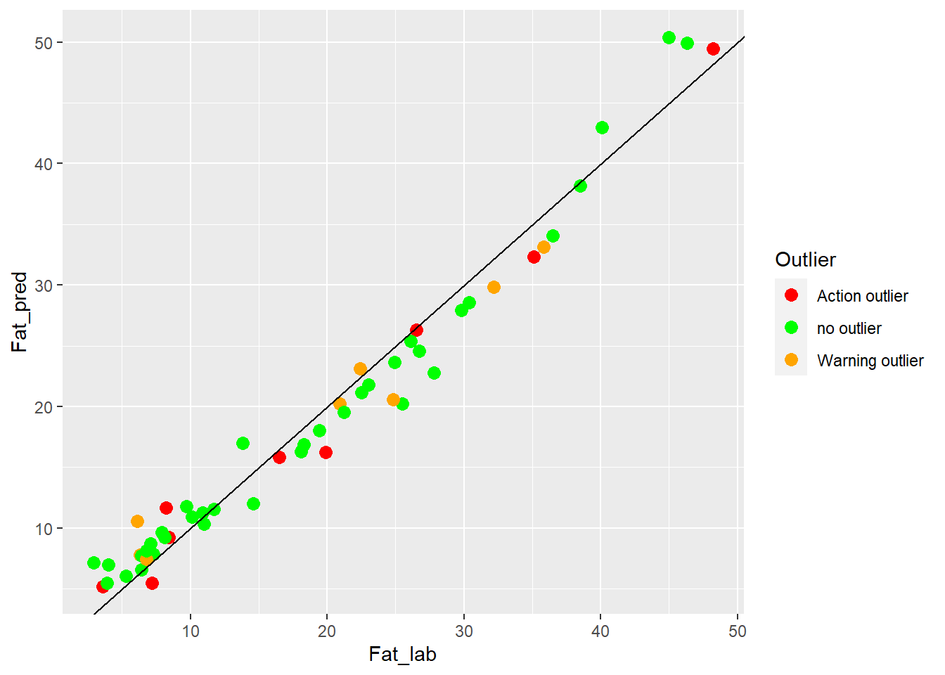
New model for Moisture
set.seed(1234)
tec2_pls_model2_moi <- train(y = tec2_moi_train$Moisture,
  x = tec2_moi_train$snvdt2der2_spec,
  method = "pls",
  tuneLength = 20,
  trControl = ctrl)

tec2_pls_model2_moi
Partial Least Squares
159 samples
100 predictors
No pre-processing
Resampling: Cross-Validated (10 fold)
Summary of sample sizes: 143, 143, 143, 143, 143, 143, ...
Resampling results across tuning parameters:
ncomp RMSE Rsquared MAE
1 1.953331 0.9638069 1.562305
2 1.910251 0.9654199 1.524954
3 1.903736 0.9670069 1.504171
4 1.876967 0.9656479 1.503045
5 1.852346 0.9663093 1.496594
6 1.818879 0.9681488 1.477183
7 1.843666 0.9665417 1.495628
8 1.989335 0.9600503 1.606336
9 2.033966 0.9573780 1.621541
10 1.996112 0.9594772 1.588339
11 2.017199 0.9591555 1.595089
12 2.259679 0.9497414 1.666685
13 2.333351 0.9430398 1.683757
14 2.413024 0.9365590 1.732497
15 2.358831 0.9382421 1.695501
16 2.401302 0.9382654 1.684079
17 2.455943 0.9288073 1.673968
18 2.513823 0.9298887 1.705269
19 2.621577 0.9261368 1.723303
20 2.814462 0.9116739 1.802853
RMSE was used to select the optimal model using the smallest value.
The final value used for the model was ncomp = 6.pls_preds2_moi <- predict(tec2_pls_model2_moi, tec2_moi_test$snvdt2der2_spec)
test_moi_preds2 <- bind_cols(tec2_moi_test$SampleID ,tec2_moi_test$Moisture, pls_preds2_moi, tec2_moi_test$outlier)
colnames(test_moi_preds2) <- c("SampleID", "Moi_lab", "Moi_pred", "Outlier")test_moi_preds2 %>%
ggplot(aes(x = Moi_lab, y = Moi_pred, colour = Outlier)) +
geom_point(size = 3) +
geom_abline() +
scale_color_manual(values = c("no outlier" = "green",
"Warning outlier" = "orange",
"Action outlier" ="red"))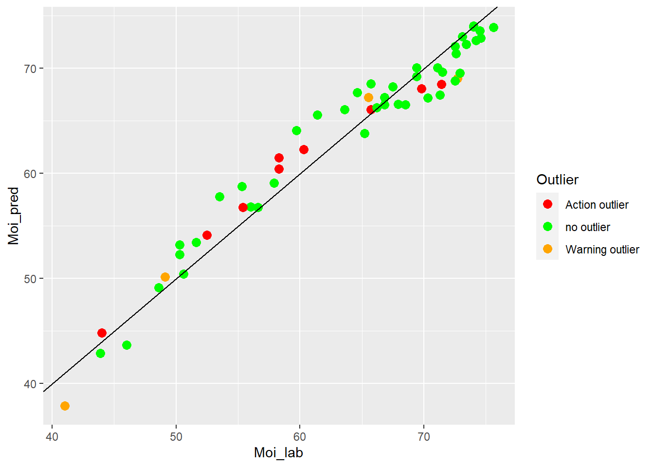
Now we can prepare a table compare the statistics for the two models:
Statistics for Model-1
| Parameter | N training | N test | Terms | C.V. error (SECV) | Test Pred. error (SEV) |
|---|---|---|---|---|---|
| Protein | 160 | 55 | 3 | 1.30 | 1.49 |
| Fat | 160 | 55 | 3 | 2.22 | 2.34 |
| Moisture | 160 | 56 | 3 | 2.01 | 2.25 |
Statistics for Model-2
| Parameter | N training | N test | Terms | C.V. error (SECV) | Test Pred. error (SEV) |
|---|---|---|---|---|---|
| Protein | 160 | 55 | 15 | 1.30 | 0.76 |
| Fat | 160 | 55 | 9 | 2.22 | 2.36 |
| Moisture | 160 | 56 | 6 | 2.01 | 2.17 |
Conclussions
We have a high improvement in the predictions of protein, but not in the models for fat and moisture, so we keep the PLS model for protein and willl continue searching an improvement for the fat and moisture parameters.