load("C:/BLOG/Workspaces/NIT Tutorial/NIT_ws14.RData")
library(tidyverse)
library(Cubist)
library(caret)Let´s continue developing regressions looking for the better performance for every parameter in our “tecator” data set. Let´s try this time with an algorithm called “Cubist”. We will use the same math treatment that we have used for the PLS, and also the same training and test sets, so this way we can compare the performance of the models. We use as well the “train” function from the “Caret” package using this time the method “cubist”.
As always we load the previous workspace
Cubist Model for Protein
set.seed(1234)
tec2_cubist_model2_prot <- train(x = tec2_prot_train$snvdt2der2_spec,
                                 y = tec2_prot_train$Protein, method = "cubist", tuneLength = 20, trControl = ctrl)

tec2_cubist_model2_prot
Cubist
160 samples
100 predictors
No pre-processing
Resampling: Cross-Validated (10 fold)
Summary of sample sizes: 144, 144, 144, 144, 144, 143, ...
Resampling results across tuning parameters:
committees neighbors RMSE Rsquared MAE
1 0 1.2870050 0.8104673 0.9534556
1 5 1.0728193 0.8699636 0.7947601
1 9 1.1102337 0.8619752 0.8147805
10 0 1.1515555 0.8506506 0.8899444
10 5 0.9585324 0.8958449 0.7263252
10 9 0.9823007 0.8913229 0.7421395
20 0 1.1560479 0.8515777 0.8868184
20 5 0.9682421 0.8945563 0.7233595
20 9 0.9884495 0.8900776 0.7365313
RMSE was used to select the optimal model using the smallest value.
The final values used for the model were committees = 10 and neighbors = 5.#summary(tec2_cubist_model2_prot)
pred_cubist_prot <- predict(tec2_cubist_model2_prot, tec2_prot_test$snvdt2der2_spec)
#plot (pred_cubist_prot, tec2_prot_test$Protein)test_cubistprot_preds <- bind_cols(tec2_prot_test$SampleID ,tec2_prot_test$Protein, pred_cubist_prot, tec2_prot_test$outlier)New names:
• `` -> `...1`
• `` -> `...2`
• `` -> `...3`
• `` -> `...4`colnames(test_cubistprot_preds) <- c("SampleID", "Prot_lab", "Prot_pred", "Outlier")test_cubistprot_preds %>%
ggplot(aes(x = Prot_pred, y = Prot_lab, colour = Outlier)) +
geom_point(size = 3) +
geom_abline() +
ggtitle("Cubist Model for Protein") +
scale_color_manual(values = c("no outlier" = "green",
"Warning outlier" = "orange",
"Action outlier" ="red"))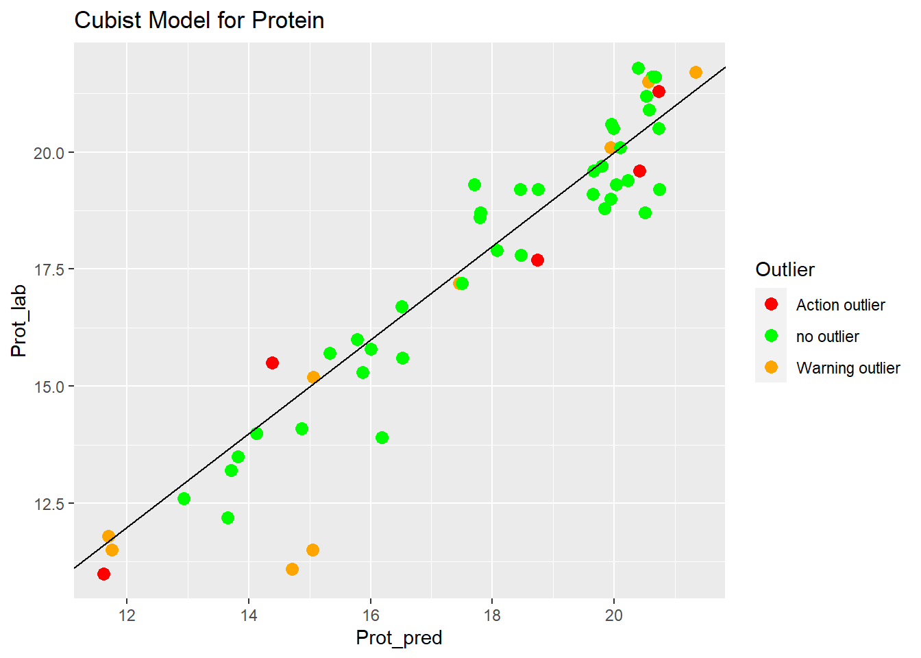
Cubist Model for Fat
set.seed(1234)
tec2_cubist_model2_fat <- train(x = tec2_fat_train$snvdt2der2_spec,
                                 y = tec2_fat_train$Fat, method = "cubist", tuneLength = 20, trControl = ctrl)

tec2_cubist_model2_fat
Cubist
160 samples
100 predictors
No pre-processing
Resampling: Cross-Validated (10 fold)
Summary of sample sizes: 144, 145, 143, 144, 144, 144, ...
Resampling results across tuning parameters:
committees neighbors RMSE Rsquared MAE
1 0 2.198035 0.9769629 1.6246736
1 5 1.083412 0.9929048 0.7781370
1 9 1.113212 0.9925964 0.8361789
10 0 2.166602 0.9782695 1.6297020
10 5 1.042068 0.9937319 0.7460829
10 9 1.078624 0.9934530 0.8008387
20 0 2.179303 0.9781454 1.6370725
20 5 1.039929 0.9937569 0.7427505
20 9 1.061908 0.9936486 0.7916956
RMSE was used to select the optimal model using the smallest value.
The final values used for the model were committees = 20 and neighbors = 5.#summary(tec2_cubist_model2_fat)
pred_cubist_fat <- predict(tec2_cubist_model2_fat, tec2_fat_test$snvdt2der2_spec)
#plot (pred_cubist_fat, tec2_fat_test$Fat)test_cubistfat_preds <- bind_cols(tec2_fat_test$SampleID ,tec2_fat_test$Fat, pred_cubist_fat, tec2_fat_test$outlier)New names:
• `` -> `...1`
• `` -> `...2`
• `` -> `...3`
• `` -> `...4`colnames(test_cubistfat_preds) <- c("SampleID", "Fat_lab", "Fat_pred", "Outlier")test_cubistfat_preds %>%
ggplot(aes(x = Fat_pred, y = Fat_lab, colour = Outlier)) +
geom_point(size = 3) +
geom_abline() +
ggtitle("Cubist Model for Fat") +
scale_color_manual(values = c("no outlier" = "green",
"Warning outlier" = "orange",
"Action outlier" ="red"))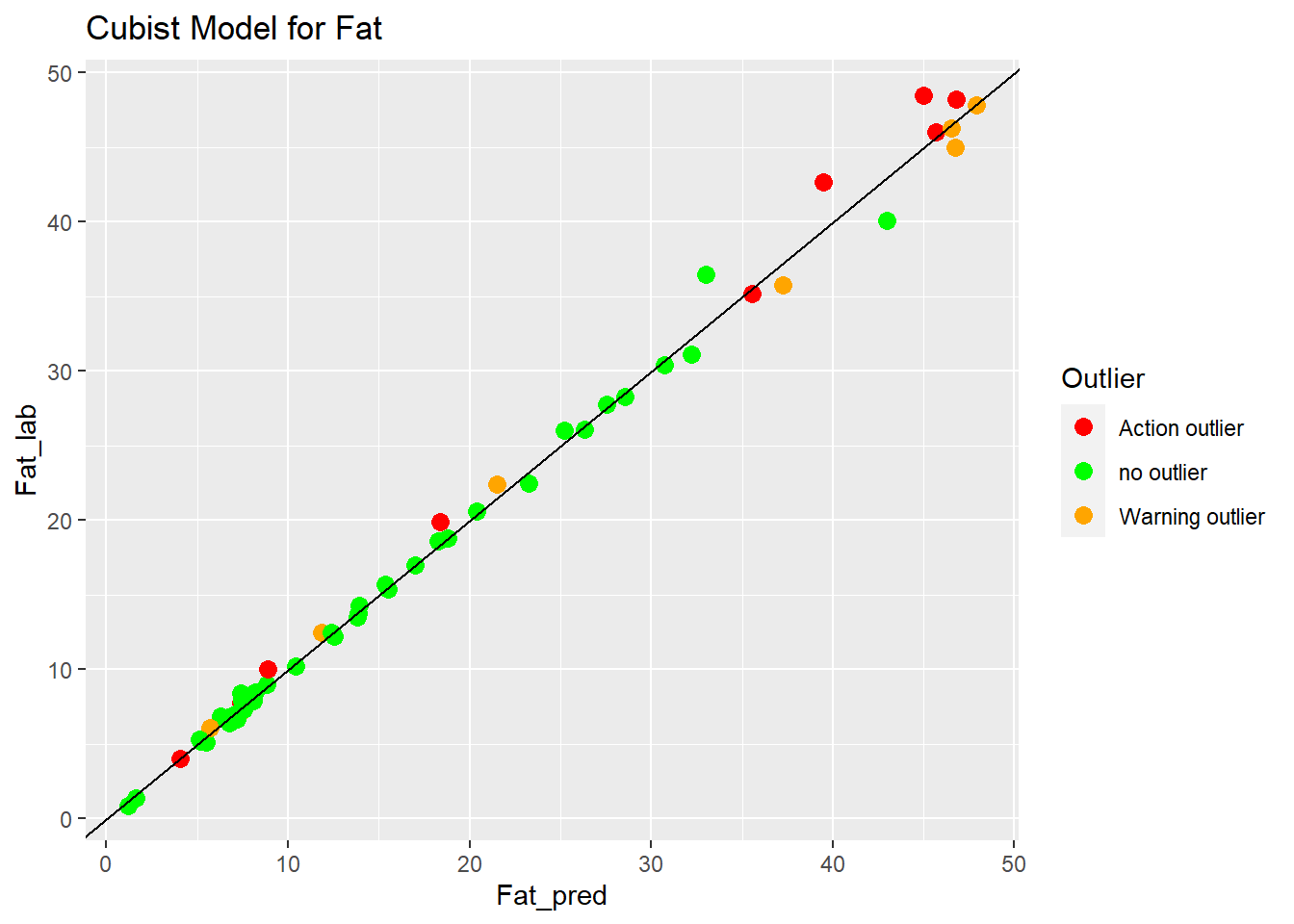
Cubist Model for Moisture
set.seed(1234)
tec2_cubist_model2_moi <- train(x = tec2_moi_train$snvdt2der2_spec,
                                 y = tec2_moi_train$Moisture, method = "cubist", tuneLength = 20, trControl = ctrl)

tec2_cubist_model2_moi
Cubist
159 samples
100 predictors
No pre-processing
Resampling: Cross-Validated (10 fold)
Summary of sample sizes: 143, 143, 143, 143, 143, 143, ...
Resampling results across tuning parameters:
committees neighbors RMSE Rsquared MAE
1 0 1.478564 0.9776294 1.1032646
1 5 1.148678 0.9846630 0.8398640
1 9 1.188129 0.9838546 0.8687294
10 0 1.426324 0.9785558 1.1171312
10 5 1.119442 0.9847117 0.8275355
10 9 1.162376 0.9838461 0.8563880
20 0 1.453163 0.9777731 1.1357573
20 5 1.137881 0.9844723 0.8375293
20 9 1.181599 0.9835126 0.8613441
RMSE was used to select the optimal model using the smallest value.
The final values used for the model were committees = 10 and neighbors = 5.#summary(tec2_cubist_model2_moi)
pred_cubist_moi <- predict(tec2_cubist_model2_moi, tec2_moi_test$snvdt2der2_spec)
#plot (pred_cubist_moi, tec2_moi_test$Moisture)test_cubistmoi_preds <- bind_cols(tec2_moi_test$SampleID ,tec2_moi_test$Moisture, pred_cubist_moi, tec2_moi_test$outlier)New names:
• `` -> `...1`
• `` -> `...2`
• `` -> `...3`
• `` -> `...4`colnames(test_cubistmoi_preds) <- c("SampleID", "Moi_lab", "Moi_pred", "Outlier")test_cubistmoi_preds %>%
ggplot(aes(x = Moi_pred, y = Moi_lab, colour = Outlier)) +
geom_point(size = 3) +
geom_abline() +
ggtitle("Cubist Model for Moisture") +
scale_color_manual(values = c("no outlier" = "green",
"Warning outlier" = "orange",
"Action outlier" ="red"))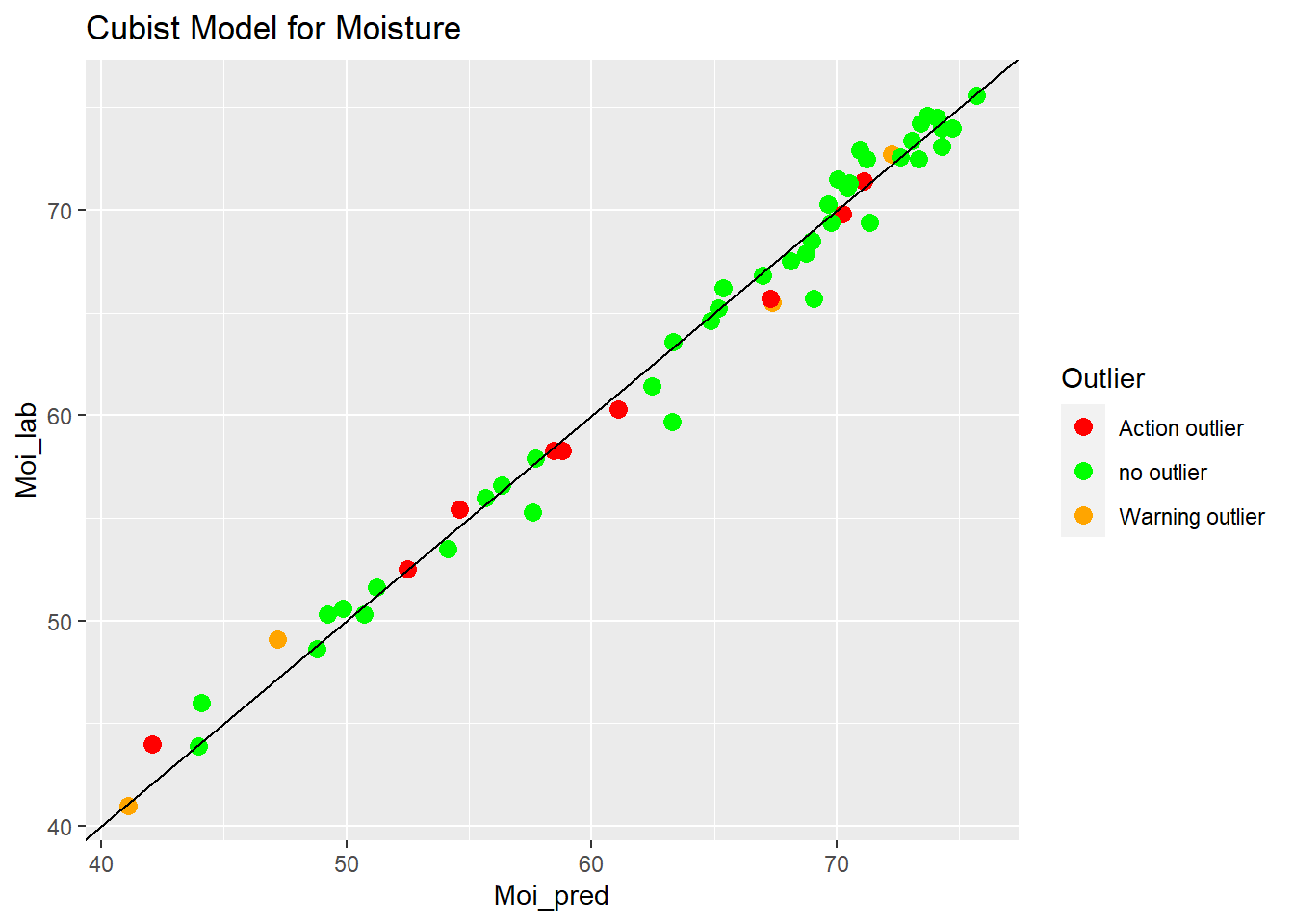
save.image("C:/BLOG/Workspaces/NIT Tutorial/NIT_ws15.RData")Statistics for the Cubist Models
| Parameter | N training | N test | Commitees | RMSE train | RMSE test |
|---|---|---|---|---|---|
| Protein | 160 | 55 | 3 | 0.96 | 1.05 |
| Fat | 160 | 55 | 1 | 0.95 | 0.75 |
| Moisture | 160 | 56 | 10 | 1.16 | 1.10 |
Conclussions
As we can see there is a high improvement in the predictions for Fat and Moisture, so it seems that in some way the cubist algorithm can handle some of the problems we saw in the pls for this two parameters. it seems that a deeper understanding of the theory of the cubist algorithm to configure better the hyper-parameters will give better models and better statistics results.