load("C:/BLOG/Workspaces/NIT Tutorial/NIT_ws15.RData")
library(tidyverse)
library(rsample)
library(randomForest)
library(caret)
library(Metrics)We continue the tutorial trying to improve as much as we can the statistics for the “tecator” data, and this time we will use the Random Forest algorithm, that is used very often with other type of data, but not with near infrared spectra data.
As always we load the previous workspace, and the libraries we need:
Random Forest model for Protein
As we have seen in other posts we have to prepare the dataframe used to build the random forest model in order not to get errors, so let´s do it first for protein:
tec2rf_prot_train <- data.frame(Protein = tec2_prot_train$Protein, tec2_prot_train$snvdt2der2_spec)
tec2rf_prot_test <- data.frame(tec2_prot_test$snvdt2der2_spec)
We are going to use cross validation to define the best hyper-parameters using the training data and keeping as always the test data apart to validate the model. Let´s divide in four folds the training data we have prepared for protein in the previous posts, and we will see how the statistics and graphics about how well the predicted values for protein fit with the reference values for every fold taken apart. Cross Validation is a good method to find outliers, and to find the best configuration for the model hyper-parameters.
# Prepare the dataframe containing the cross validation partitions
t2prot_cv_split <- vfold_cv(tec2rf_prot_train, v = 4)
t2prot_cv_data <- t2prot_cv_split %>%
  mutate(
    # Extract the train dataframe for each split
    train = map(splits, ~training(.x)),
    # Extract the validate dataframe for each split
    validate = map(splits, ~testing(.x))
  )
# Use head() to preview cv_data
head(t2prot_cv_data)
# 4-fold cross-validation
# A tibble: 4 × 4
splits id train validate
<list> <chr> <list> <list>
1 <split [120/40]> Fold1 <df [120 × 101]> <df [40 × 101]>
2 <split [120/40]> Fold2 <df [120 × 101]> <df [40 × 101]>
3 <split [120/40]> Fold3 <df [120 × 101]> <df [40 × 101]>
4 <split [120/40]> Fold4 <df [120 × 101]> <df [40 × 101]>Now we have the data prepared to develop the regression:
# Build a random forest model for each fold
t2prot_cv_models_rf <- t2prot_cv_data %>%
  mutate(model = map(train, ~randomForest(formula = Protein ~.,
                     data = .x, num.trees = 500)))

t2prot_cv_prep_rf <- t2prot_cv_models_rf %>%
  mutate(
    # Extract the recorded CaCO3 for the records in the validate dataframes
    validate_actual = map(validate, ~.x$Protein),
    # Predict Clay for each validate set using its corresponding model
    validate_predicted = map2(.x = model, .y = validate, ~predict(.x, .y))
  )


# Calculate validate MAE for each fold
t2prot_cv_eval_rf <- t2prot_cv_prep_rf %>%
  mutate(validate_rmse = map2_dbl(validate_actual, validate_predicted, ~rmse(actual = .x, predicted = .y)))

# Print the validate_rmse column
t2prot_cv_eval_rf$validate_rmse
[1] 1.0805879 0.9528476 0.7627112 1.0173726# Calculate the mean of validate_mae column
mean(t2prot_cv_eval_rf$validate_rmse)[1] 0.9533799As we see the RMSE does not improve the value for the PLS
For a better visualization we create a dataframe with the actual values and predictions for the four folds, creating a new field to add the fold value.
cv_fold1 <- bind_cols(t2prot_cv_eval_rf$id[[1]],
                      t2prot_cv_eval_rf$validate_actual[[1]],
                      t2prot_cv_eval_rf$validate_predicted[[1]])
New names:
• `` -> `...1`
• `` -> `...2`
• `` -> `...3`cv_fold1 <- cv_fold1 %>%
mutate(Fold = "Fold 1")
cv_fold2 <- bind_cols(t2prot_cv_eval_rf$id[[2]],
t2prot_cv_eval_rf$validate_actual[[2]],
t2prot_cv_eval_rf$validate_predicted[[2]])New names:
• `` -> `...1`
• `` -> `...2`
• `` -> `...3`cv_fold2 <- cv_fold2 %>%
mutate(Fold = "Fold 2")
cv_fold3 <- bind_cols(t2prot_cv_eval_rf$id[[3]],
t2prot_cv_eval_rf$validate_actual[[3]],
t2prot_cv_eval_rf$validate_predicted[[3]])New names:
• `` -> `...1`
• `` -> `...2`
• `` -> `...3`cv_fold3 <- cv_fold3 %>%
mutate(Fold = "Fold 3")
cv_fold4 <- bind_cols(t2prot_cv_eval_rf$id[[4]],
t2prot_cv_eval_rf$validate_actual[[4]],
t2prot_cv_eval_rf$validate_predicted[[4]])New names:
• `` -> `...1`
• `` -> `...2`
• `` -> `...3`cv_fold4 <- cv_fold4 %>%
mutate(Fold = "Fold 4")
cv_rf_evaluation <- bind_rows(cv_fold1, cv_fold2, cv_fold3, cv_fold4)
colnames(cv_rf_evaluation) <- c("ID", "Actual", "Predicted", "Fold")
unique(cv_rf_evaluation$ID)[1] "Fold1" "Fold2" "Fold3" "Fold4"cv_rf_evaluation %>%
ggplot( aes(x = Predicted, y = Actual, colour = Fold)) +
geom_point() +
facet_wrap(~Fold)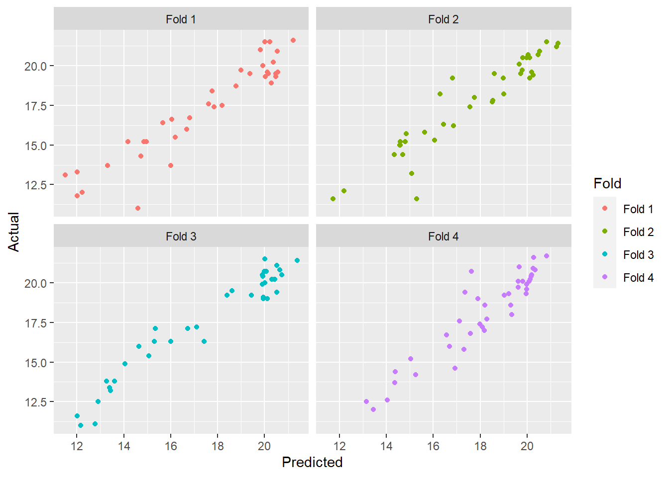
In the next posts we will try to fin a better tuning if possible.