load("C:/BLOG/Workspaces/NIT Tutorial/NIT_ws9.RData")First of all let´s load the previous workspace:
and the libraries that we are going to use:
library(chemometrics)
library(resemble)
library(scatterplot3d)
In this post we start looking for outiers, or samples which look different than the majority. Finally we have decided to select three principal components, for that reason is much easier the graphical representation due to we can use 2D or 3D graphics. One of the most common methods is to draw an ellipsoid in the Principal Component space and the samples which fall outside the ellipsoid are considered as outliers.
As we remember the score matrix is tecator_pc$x[ , 1:3], and we can see all the posible scores planes with:
pairs(tecator_pc$x[ ,1:3])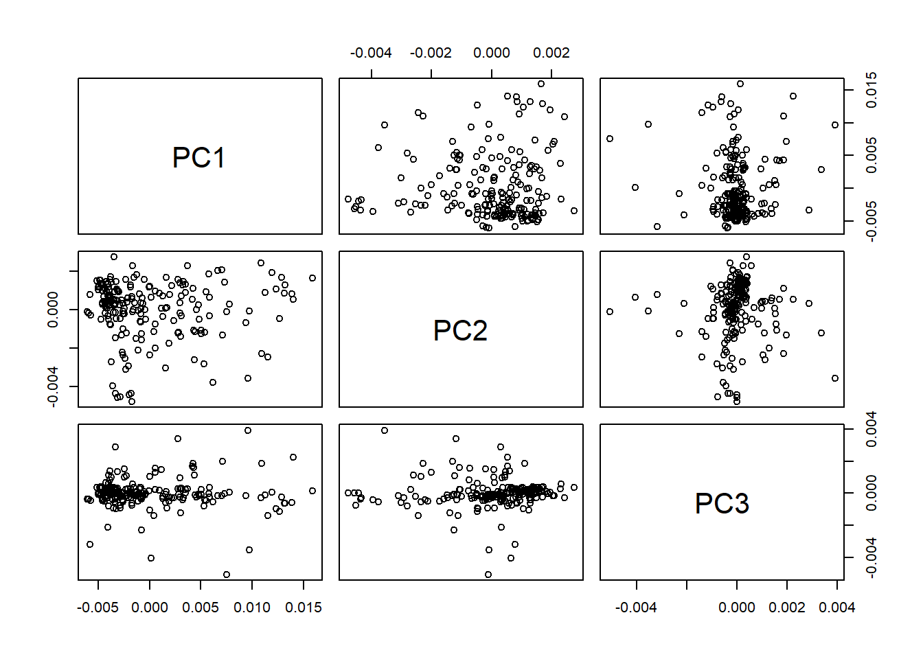
Mahalanobis distances ellipses
We can create ellipses on every plane with the average spectrum in the center. As we can see the ratio change depending of the PC number and its variability.
drawMahal(tecator_pc$x[ , 1:2], center = apply(tecator_pc$x[ , 1:2], 2, mean),
          covariance = cov(tecator_pc$x[ , 1:2]), quantile = 0.975 )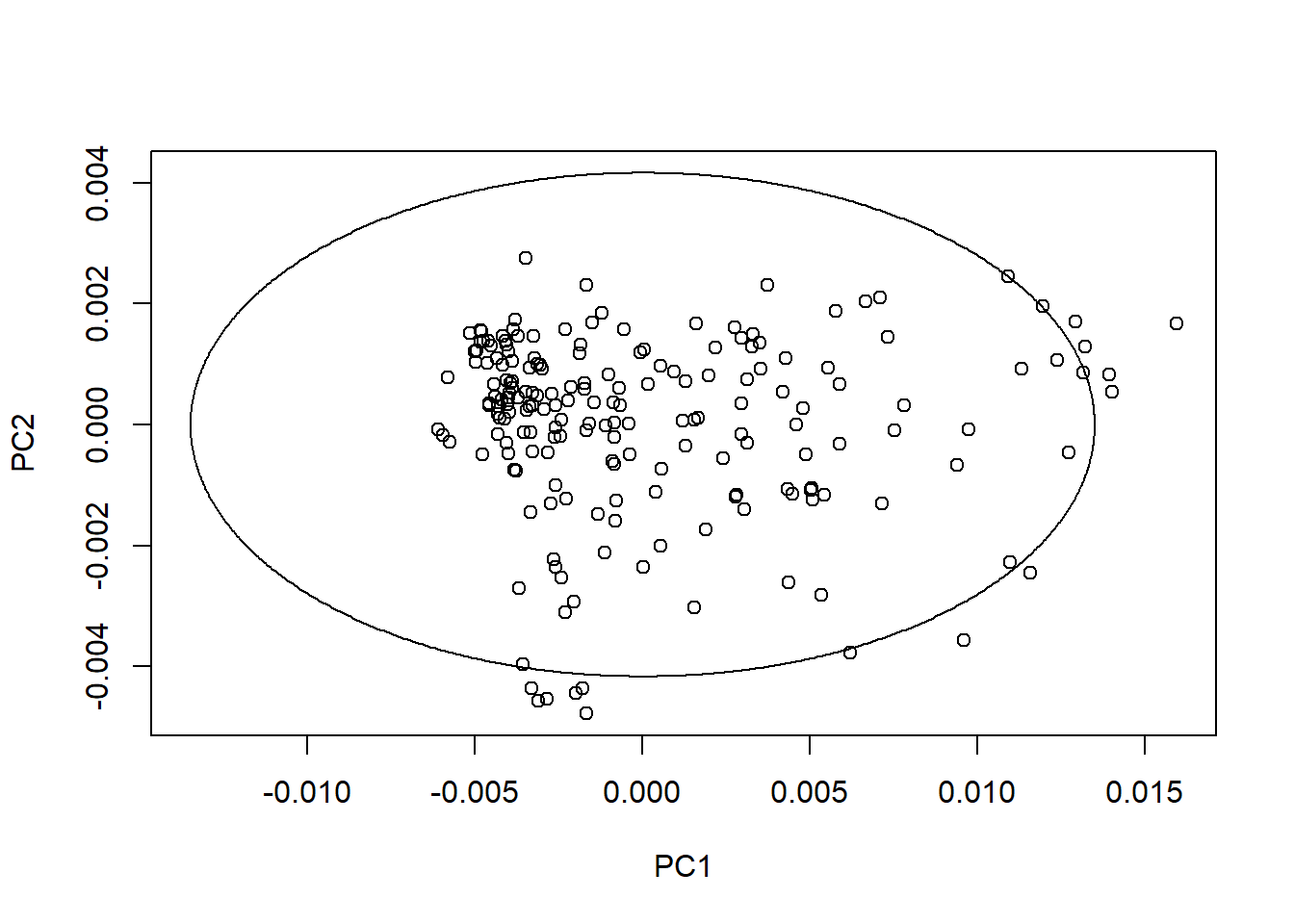
drawMahal(tecator_pc$x[ , c(1,3)], center = apply(tecator_pc$x[ , c(1,3)], 2, mean),
          covariance = cov(tecator_pc$x[ , c(1,3)]), quantile = 0.975 )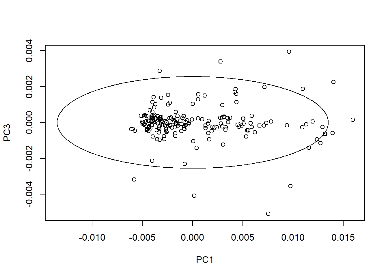
drawMahal(tecator_pc$x[ , c(2,3)], center = apply(tecator_pc$x[ , c(2,3)], 2, mean),
          covariance = cov(tecator_pc$x[ , c(2,3)]), quantile = 0.975 )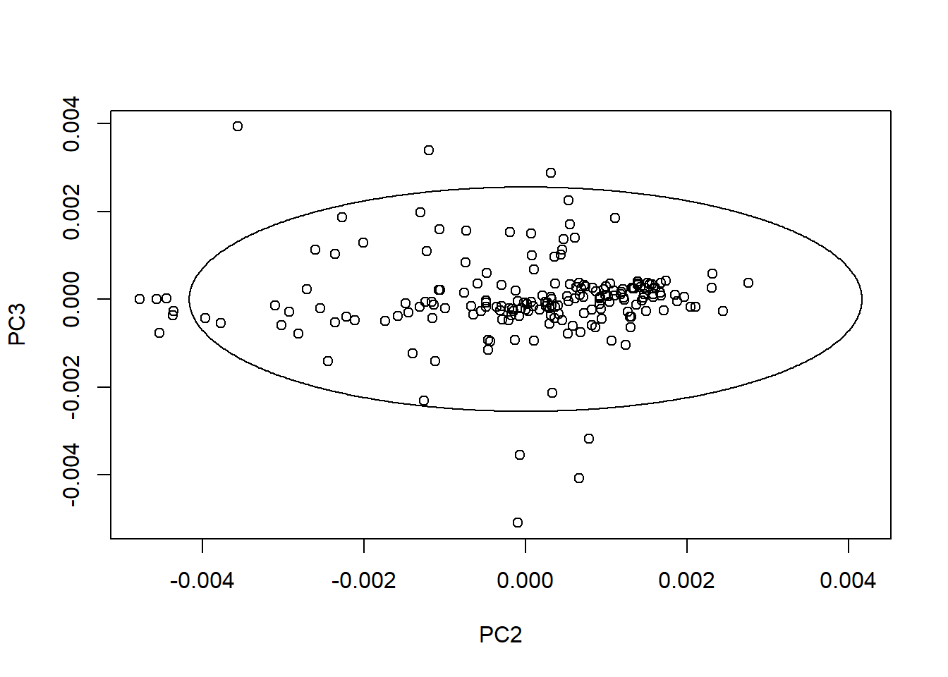
The final Mahalanobis distance is calculated for the three principal components, so we have to proceed with a calculation which use the complete score matrix (the three PC selected). Let`s keep the distances (classical and robust) value in an object called “res”.
res <- Moutlier(tecator_pc$x[ , 1:3])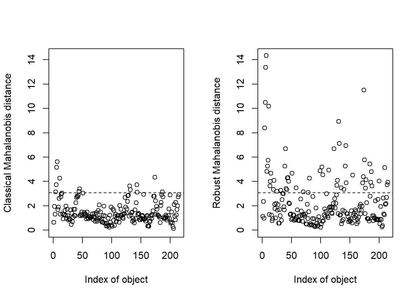
Now we can take apart the samples with distance higher than 3, and make a subset with them:
md_out <-  which(res$md > 3)
md_out <- tecator_pc$x[md_out, ]
Looking to the mahalanobis distance outliers
Let`s mark these outlier samples in the ellipses we have seen before:
drawMahal(tecator_pc$x[ , 1:2], center = apply(tecator_pc$x[ , 1:2], 2, mean),
          covariance = cov(tecator_pc$x[ , 1:2]), quantile = 0.975, col = "grey" )

points(x = md_out[ , 1],
       y = md_out[ , 2],
       pch = 16,
       col = "red")

text(md_out[ , 1], md_out[ , 2], label = rownames(md_out), pos = 2)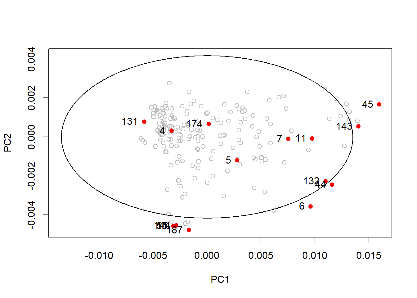
As we can see in this first plot many of the samples with hight Mahalanobis distance are inside the ellipse (131, 4, 174, 5, 7, 11, 132 and 44)
drawMahal(tecator_pc$x[ , c(1,3)], center = apply(tecator_pc$x[ , c(1,3)], 2, mean),
          covariance = cov(tecator_pc$x[ , c(1,3)]), quantile = 0.975, col = "grey" )

points(x = md_out[ , 1],
       y = md_out[ , 3],
       pch = 16,
       col = "red")

text(md_out[ , 1], md_out[ , 3], label = rownames(md_out), pos = 2)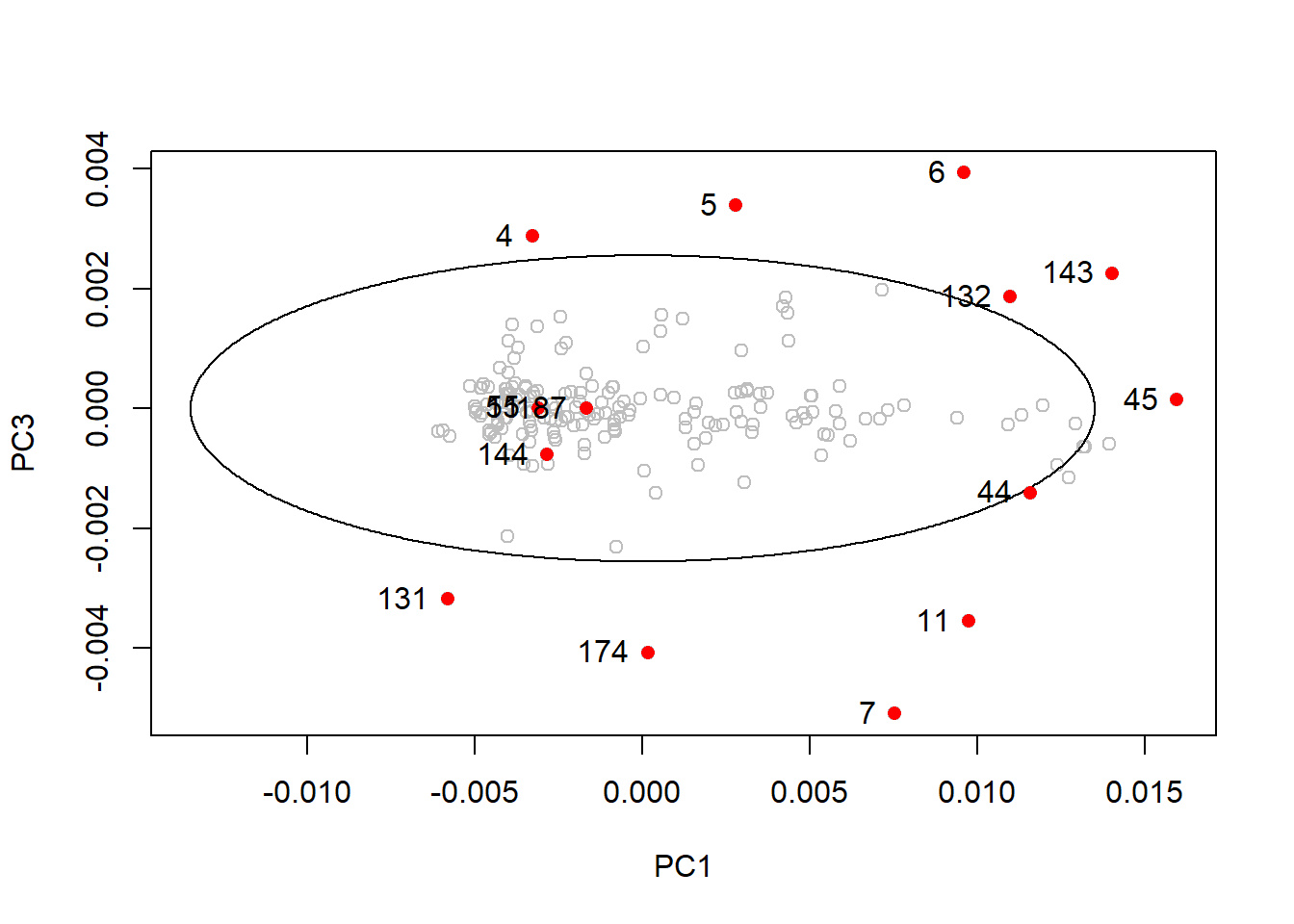
In this plot all the samples that were into the ellipse on the first plot are now outside.
drawMahal(tecator_pc$x[ , c(2,3)], center = apply(tecator_pc$x[ , c(2,3)], 2, mean),
          covariance = cov(tecator_pc$x[ , c(2,3)]), quantile = 0.975, col = "grey" )
points(x = md_out[ , 2],
       y = md_out[ , 3],
       pch = 16,
       col = "red")
text(md_out[ , 2], md_out[ , 3], label = rownames(md_out), pos = 2)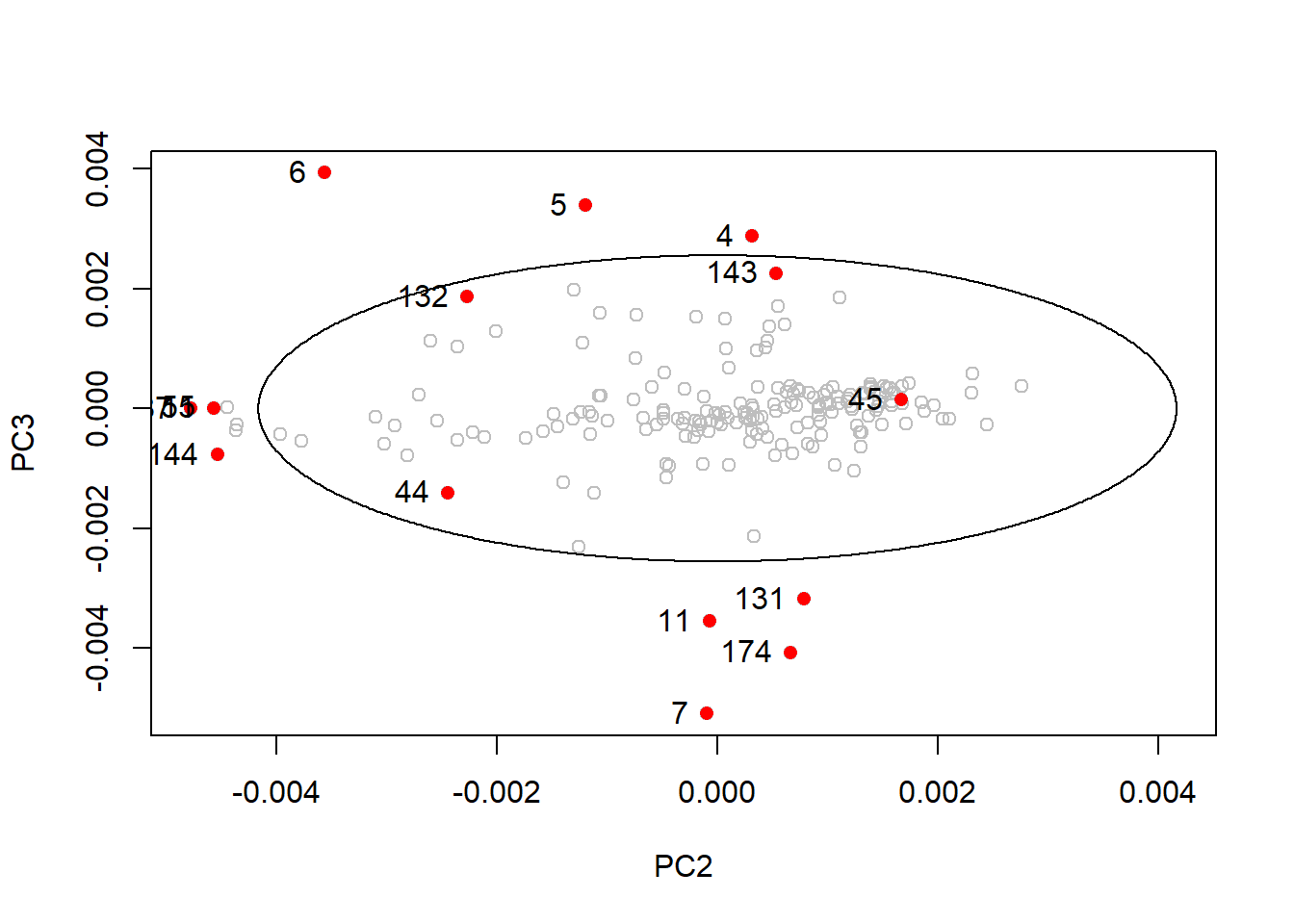
Looking to cubes in 3D
On the third plot again same samples are on and other out, so we have to take into acount that the Mahalanobis distance is a combination distance of the three planes, so we have to look at all of them at the same time and the better way to do it (in the case of three PCs), is in a cube.
tecator_pc_3d <- scatterplot3d(tecator_pc$x[ , 1],
              tecator_pc$x[ , 2],
              tecator_pc$x[ , 3],
              xlab = "PC1",
              ylab = "PC2",
              zlab = "PC3",
              color = rgb(red=0.5, green=0.5, blue=0.5, alpha = 0.5),
              pch = 16, angle =50)

tecator_pc_3d$points3d(md_out[ , 1],
                       md_out[ , 2],
                       md_out[ , 3],
                       pch = "X",
                       col = "red")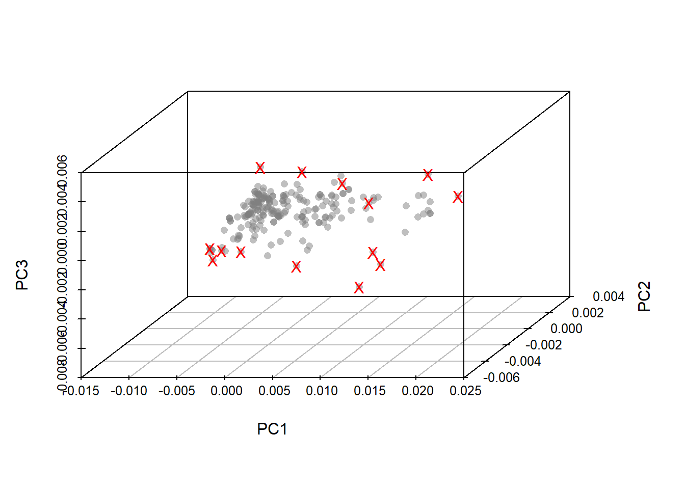
Note
I have been working with the software Win ISI (used develop models for Foss NIR Systems) for a long time, and developing the PCA with a similar math treatment, we get the same Mahalanobis distance robust outliers than our calculation with the chemometric package.
let`s save the workspace for our next post
save.image("C:/BLOG/Workspaces/NIT Tutorial/NIT_ws10.RData")