PCA - NIT tutorial (part 11)

The first idea for this post is to add a new variable with the robust Mahalanobis distance value we have obtained in the previous post. From this variable, we create a new factor variable to define three types of samples: “no H outlier” for the samples with a robust mahalanobis distance lower than 3, “Warning H outlier” for the samples with values betweeen 3 and 4, and “Action H outlier” for the samples with values higher than 4..

Let`s start by loading our workspace and the libraries we are going to use:

load("C:/BLOG/Workspaces/NIT Tutorial/NIT_ws10.RData")
library(tidyverse)

As we are going to work from now with the spectra math treated with scatter correction and second derivative, we can create a new dataframe with this spectra data, the reference values and other user defined fields that we can consider as the robust mahalanobis distance we have been talking before.

tecator1 <- 
tecator %>% 
  select(SampleID, Moisture, Fat, Protein, snvdt2der2_spec) %>% 
  mutate(RMD = as.numeric(res$rd))

Now let`s add the new variable with the robust mahalanobis distances. Normally, if the distances are below 3 the samples are not considered as outliers, if they are between 3 and 4 are considered as warning outliers and if they are over 4, they are considered as action outliers. it is important to know if the outliers have some relation with extreme reference values (for every parameter) or any other variables like the origin, temperature, instrument (in case we have more than one in our database), etc. Let´s add a new factor variable to define if the samples are “no ourliers”, “warning ourliers” or “action outliers”.

tecator2 <- 
tecator1 %>% 
  #define new variable 'scorer' using mutate() and case_when()
  mutate(outlier = case_when(RMD <= 3 ~ "no outlier",
                           RMD > 3 & RMD <= 4 ~ "Warning outlier",
                           RMD > 4 ~ "Action outlier")) %>% 
  mutate(outlier = as.factor(outlier))

before to develop the regressions, why not to see if the outliers are related to extreme samples for the different parameters. We can see that giving colors to the histograms to the histograms (for example). So let`s plot the histograms for the tecator parameters ( moisture, fat and protein)

Histograms for moisture with Mahalanobis ranges colors.

ggplot(tecator2, aes(x = Moisture, fill = outlier)) + 
  geom_histogram(position = "identity", alpha = 1, bins = 50) +
  scale_fill_manual(values = c("no outlier" = "green",
                                "Warning outlier" = "orange",
                                "Action outlier" ="red"))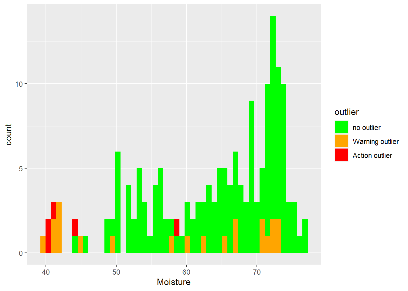

Histograms for fat with Mahalanobis ranges colors.

ggplot(tecator2, aes(x = Fat, fill = outlier)) +                 
  geom_histogram(position = "identity", alpha = 1, bins = 50) +
  scale_fill_manual(values = c("no outlier" = "green",
                                "Warning outlier" = "orange",
                                "Action outlier" ="red"))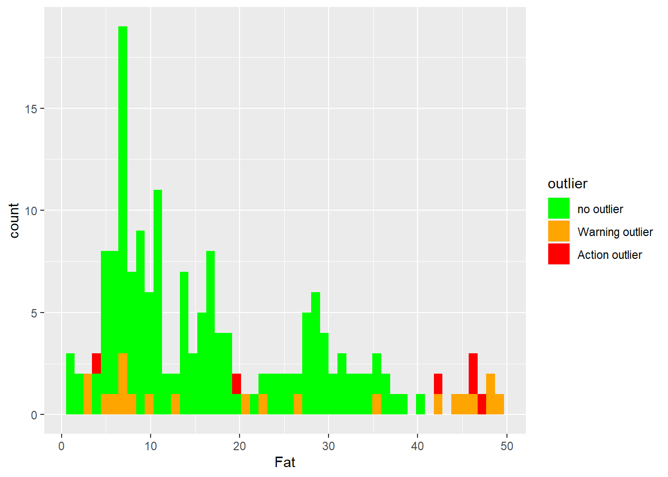

Histograms for protein with Mahalanobis ranges colors.

ggplot(tecator2, aes(x = Protein, fill = outlier)) +
  geom_histogram(position = "identity", alpha = 1, bins = 50) +
  scale_fill_manual(values = c("no outlier" = "green",
                                "Warning outlier" = "orange",
                                "Action outlier" ="red"))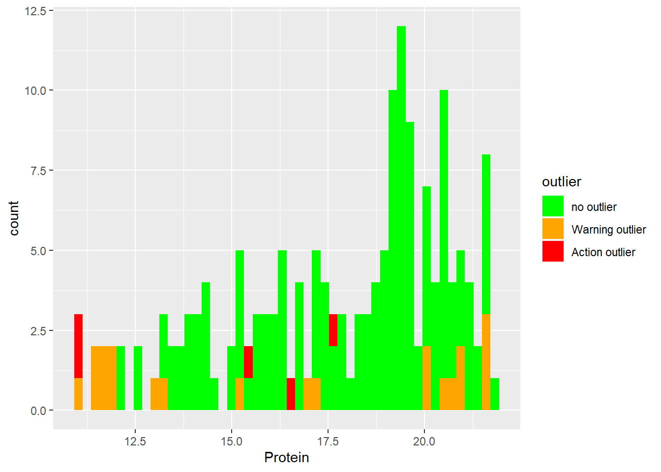

As we can see extreme samples are normally warning or action outliers (we can confirm this better when we will develop the regressions on coming posts), but there are other causes as well.

let`s save the workspace for our next post

save.image("C:/BLOG/Workspaces/NIT Tutorial/NIT_ws11.RData")