load("C:/BLOG/Workspaces/NIT Tutorial/NIT_ws16.RData")
library(tidyverse)
library(caret)
library(earth)
library(Monitor)Let´s load first the previous workspace and the libraries needed.
We all have listen about Support Vector Machines algorithm to build Chemometric models, but I never try to do it , so this tutorial is a good opportunity to try. I use Caret package and use a default procedure described in the book “Applied Predictive Modeling”, so we know that there is margin for improvement with other configurations.
As always we develop the model with the samples selected for training and validate eith the samples taken apart for testing.
SVM model for Protein
set.seed(100)
svm_tec_prot <- train(x = tec2_prot_train$snvdt2der2_spec, y = tec2_prot_train$Protein,
                       method = "svmRadial",
                       tuneLength = 14,
                       preproc = c("center", "scale"),
                       trControl = trainControl(method = "cv"))
svm_protpreds <- predict(svm_tec_prot, tec2_prot_test$snvdt2der2_spec)
test_prot_svmpreds <- bind_cols(tec2_prot_test$SampleID ,tec2_prot_test$Protein, svm_protpreds)
colnames(test_prot_svmpreds) <- c("SampleID", "Prot_lab", "Prot_pred")
test_prot_svmpreds %>%
ggplot( aes(x = Prot_pred, y = Prot_lab)) +
geom_point()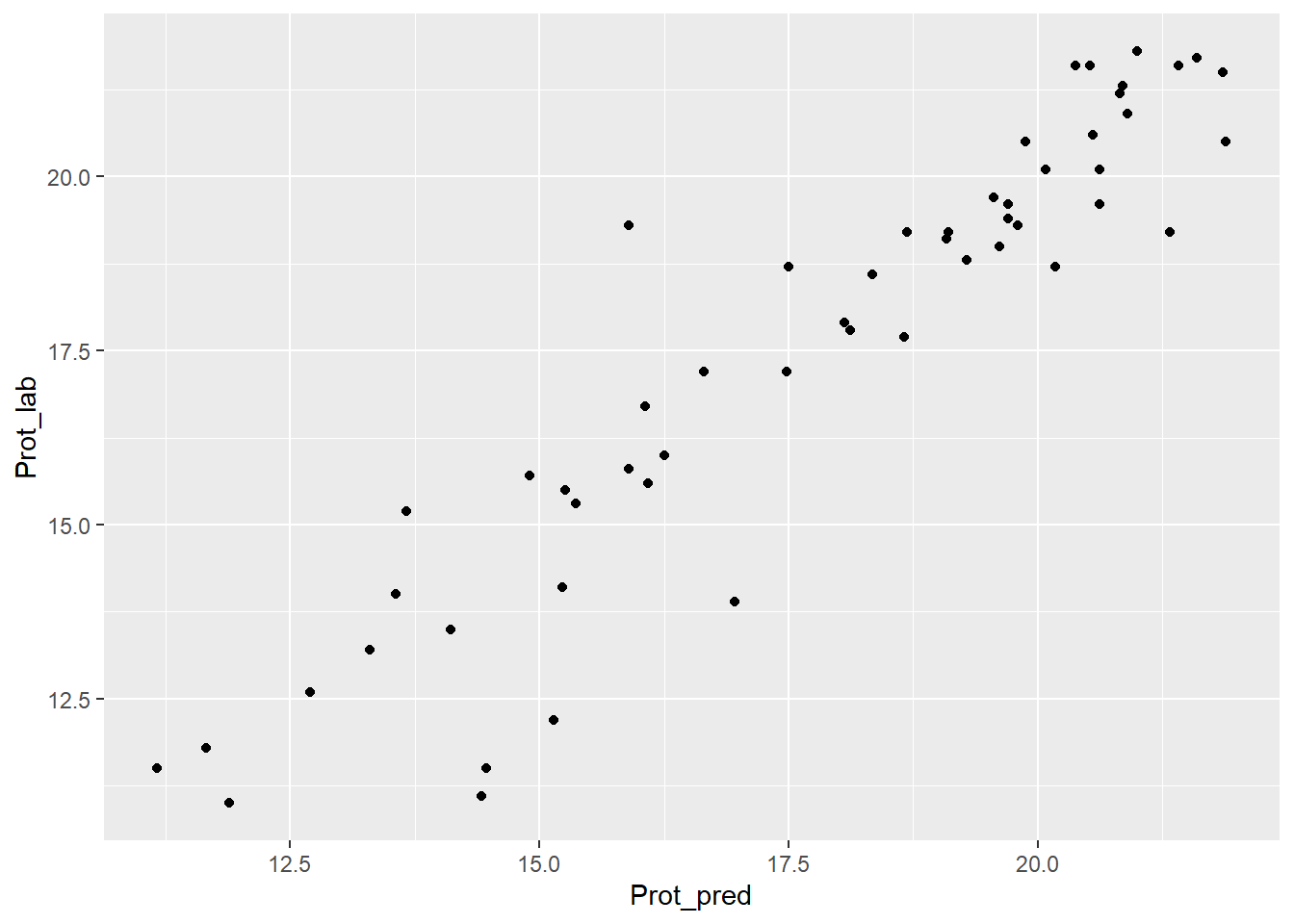
Let´s use the Monitor package to see the statistics:
monitor_xyplot(test_prot_svmpreds[ , 1:3])Validation Samples = 55
Reference Mean = 17.59455
Predicted Mean = 17.79309
RMSEP : 1.16366
Bias : -0.1985454
SEP : 1.157165
Corr : 0.9356546
RSQ : 0.8754495
Slope : 1.022215
Intercept : -0.5938104
*** Std Dev of the model not supplied, RPD not calculated ***
*** Details of the model used for prediction not supplied ***
*** SEP significance not calculated ***
Residual Std Dev is : 1.17
***Slope/Intercept adjustment in not necessary***
Bias : -0.1985454
SEP : 1.157165
BCL(+/-) : 0.3126953
BCL percentage: 31.26953
***Bias adjustment in not necessary***
Without any adjustment and using SEP as std dev the residual distibution is:
Residuals into 68% prob (+/- 1SEP) = 44 % = 80
Residuals into 95% prob (+/- 2SEP) = 50 % = 90.90909
Residuals into 99.5% prob (+/- 3SEP) = 55 % = 100
Residuals outside 99.5% prob (+/- 3SEP) = 0 % = 0 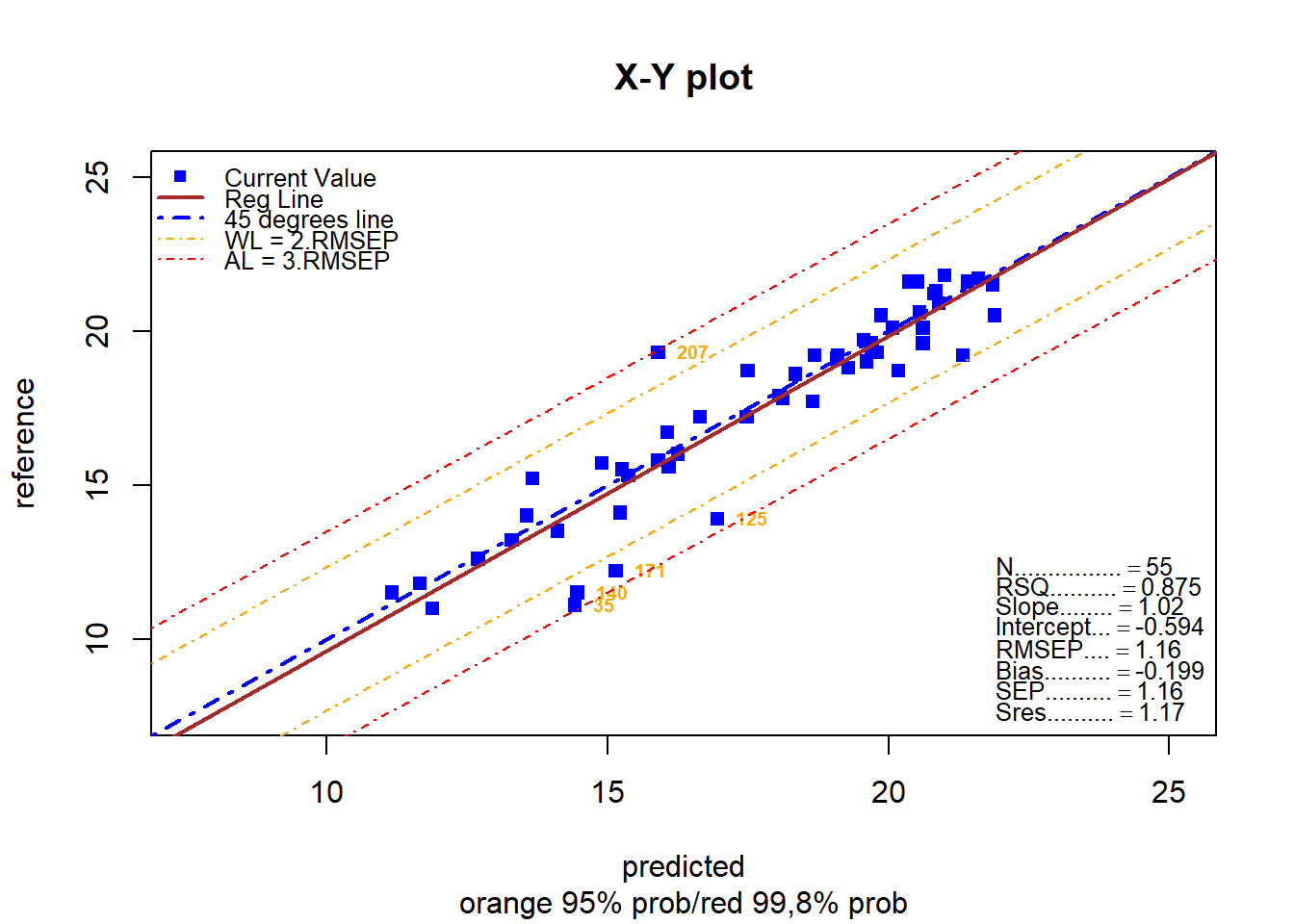
$ResWarning
   index  id  ref     pred       res res.corr1 res.corr2          Q   Color
12    12  35 11.1 14.42107 -3.321071     -3.12     -3.05 Q1 to MIN  #0000FF
36    36 125 13.9 16.95782 -3.057816     -2.86     -2.84 Q1 to MIN  #0000FF
39    39 140 11.5 14.46377 -2.963773     -2.77     -2.69 Q1 to MIN  #0000FF
47    47 171 12.2 15.14471 -2.944707     -2.75     -2.69 Q1 to MIN  #0000FF
55    55 207 19.3 15.89985  3.400155      3.60      3.64         Q2 #FFFF33

$ResWarningList
[1] 12 36 39 47 55

$ResAction
[1] index     id        ref       pred      res       res.corr1 res.corr2
[8] Q         Color
<0 rows> (or 0-length row.names)

$ResActionList
numeric(0)
SVM model for Fat
set.seed(100)
svm_tec_fat <- train(x = tec2_prot_train$snvdt2der2_spec, y = tec2_prot_train$Fat,
                       method = "svmRadial",
                       tuneLength = 14,
                       preproc = c("center", "scale"),
                       trControl = trainControl(method = "cv"))
svm_fatpreds <- predict(svm_tec_fat, tec2_fat_test$snvdt2der2_spec)
test_fat_svmpreds <- bind_cols(tec2_fat_test$SampleID ,tec2_fat_test$Fat, svm_fatpreds)
colnames(test_fat_svmpreds) <- c("SampleID", "Fat_lab", "Fat_pred")
test_fat_svmpreds %>%
ggplot( aes(x = Fat_pred, y = Fat_lab)) +
geom_point()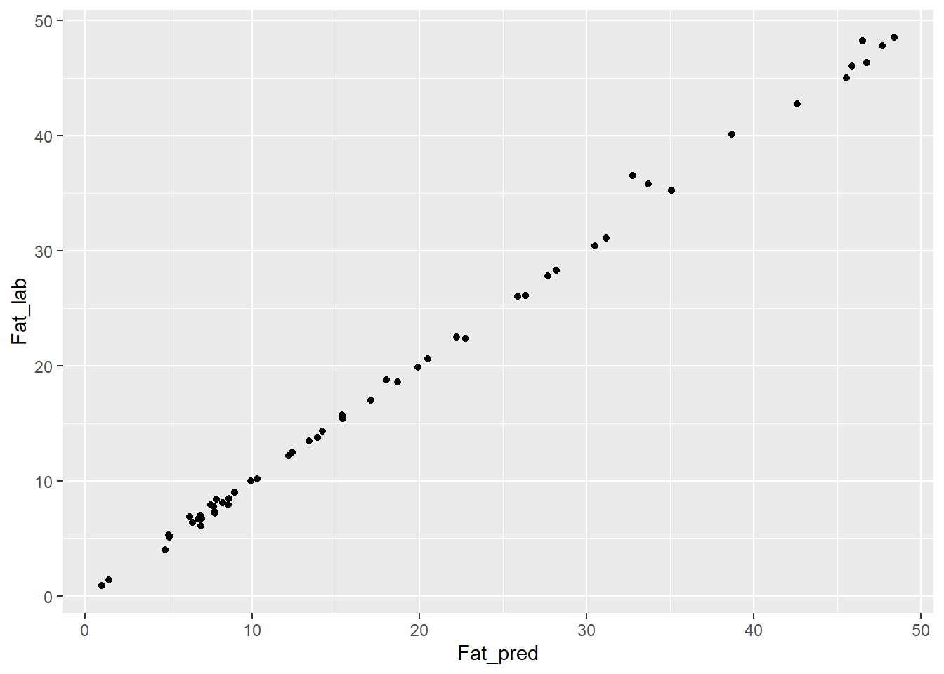
Let´s use the Monitor package to see the statistics:
monitor_xyplot(test_fat_svmpreds[ , 1:3])Validation Samples = 55
Reference Mean = 19.01091
Predicted Mean = 18.87002
RMSEP : 0.7133293
Bias : 0.1408927
SEP : 0.7057218
Corr : 0.9988758
RSQ : 0.9977529
Slope : 1.014583
Intercept : -0.1342866
*** Std Dev of the model not supplied, RPD not calculated ***
*** Details of the model used for prediction not supplied ***
*** SEP significance not calculated ***
Residual Std Dev is : 0.68
***Slope/Intercept adjustment is recommended***
Bias : 0.1408927
SEP : 0.7057218
BCL(+/-) : 0.1907039
BCL percentage: 19.07039
***Bias adjustment in not necessary***
Without any adjustment and using SEP as std dev the residual distibution is:
Residuals into 68% prob (+/- 1SEP) = 48 % = 87.27273
Residuals into 95% prob (+/- 2SEP) = 52 % = 94.54545
Residuals into 99.5% prob (+/- 3SEP) = 54 % = 98.18182
Residuals outside 99.5% prob (+/- 3SEP) = 1 % = 1.818182 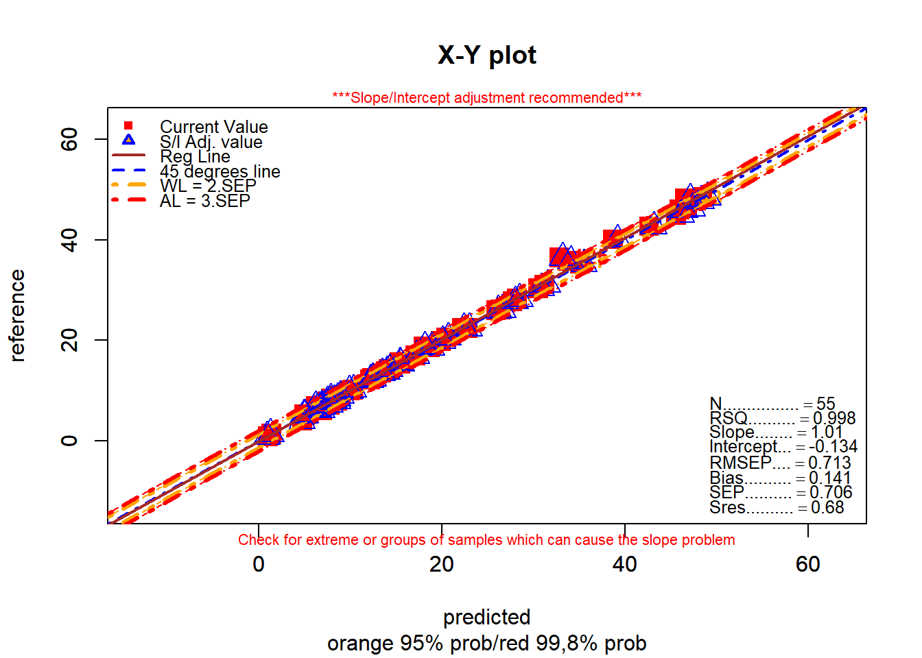
With S/I correction and using Sres as standard deviation, the Residual Distribution would be:
  Residuals into 68%   prob (+/- 1Sres)     = 47     % = 85.45455
  Residuals into 95%   prob (+/- 2Sres)     = 53     % = 96.36364
  Residuals into 99.5% prob (+/- 3Sres)     = 54    % = 98.18182
  Residuals outside  99.5% prob (> 3Sres)   = 1     % = 1.818182
$ResWarning
index id ref pred res res.corr1 res.corr2 Q Color
13 13 41 35.8 33.69096 2.109041 1.97 1.75 Q2 to MAX #FF9933
14 14 43 48.2 46.52586 1.674137 1.53 1.13 Q2 to MAX #FF9933
$ResWarningList
[1] 13 14
$ResAction
index id ref pred res res.corr1 res.corr2 Q Color
33 33 125 36.5 32.79654 3.703458 3.56 3.36 Q2 to MAX #FF9933
$ResActionList
[1] 33SVM model for Moisture
set.seed(100)
svm_tec_moi <- train(x = tec2_moi_train$snvdt2der2_spec, y = tec2_moi_train$Moisture,
                       method = "svmRadial",
                       tuneLength = 14,
                       preproc = c("center", "scale"),
                       trControl = trainControl(method = "cv"))
svm_moipreds <- predict(svm_tec_moi, tec2_moi_test$snvdt2der2_spec)
test_moi_svmpreds <- bind_cols(tec2_moi_test$SampleID ,tec2_moi_test$Moisture, svm_moipreds)
colnames(test_moi_svmpreds) <- c("SampleID", "Moisture_lab", "Moisture_pred")
test_moi_svmpreds %>%
ggplot( aes(x = Moisture_pred, y = Moisture_lab)) +
geom_point()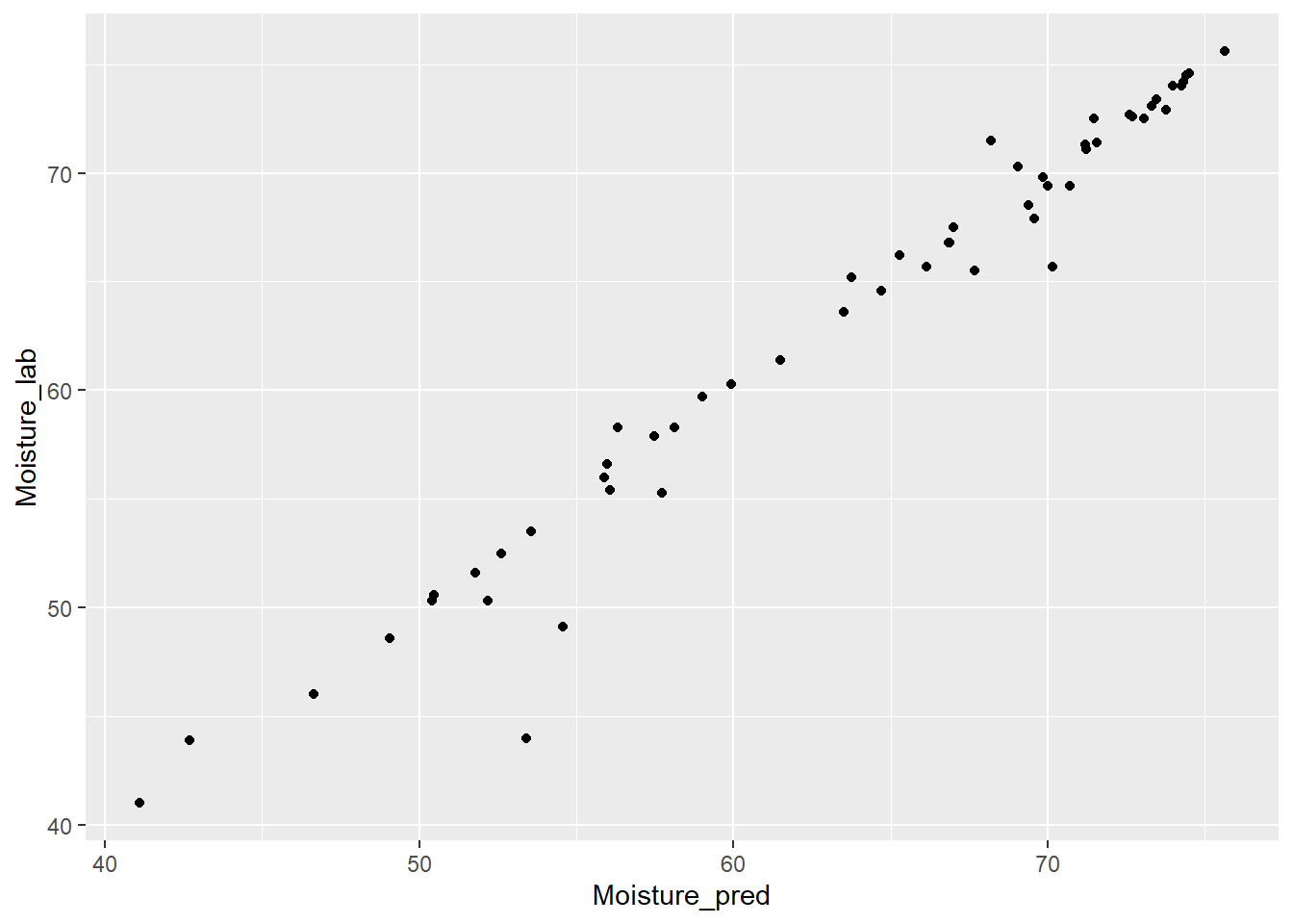
Let´s use the Monitor package to see the statistics:
monitor_xyplot(test_moi_svmpreds[ , 1:3])Validation Samples = 56
Reference Mean = 63.3625
Predicted Mean = 63.75773
RMSEP : 1.815258
Bias : -0.3952311
SEP : 1.787743
Corr : 0.9830242
RSQ : 0.9663366
Slope : 1.020187
Intercept : -1.682337
*** Std Dev of the model not supplied, RPD not calculated ***
*** Details of the model used for prediction not supplied ***
*** SEP significance not calculated ***
Residual Std Dev is : 1.79
***Slope/Intercept adjustment in not necessary***
Bias : -0.3952311
SEP : 1.787743
BCL(+/-) : 0.4785686
BCL percentage: 47.85686
***Bias adjustment in not necessary***
Without any adjustment and using SEP as std dev the residual distibution is:
Residuals into 68% prob (+/- 1SEP) = 48 % = 85.71429
Residuals into 95% prob (+/- 2SEP) = 53 % = 94.64286
Residuals into 99.5% prob (+/- 3SEP) = 54 % = 96.42857
Residuals outside 99.5% prob (+/- 3SEP) = 2 % = 3.571429 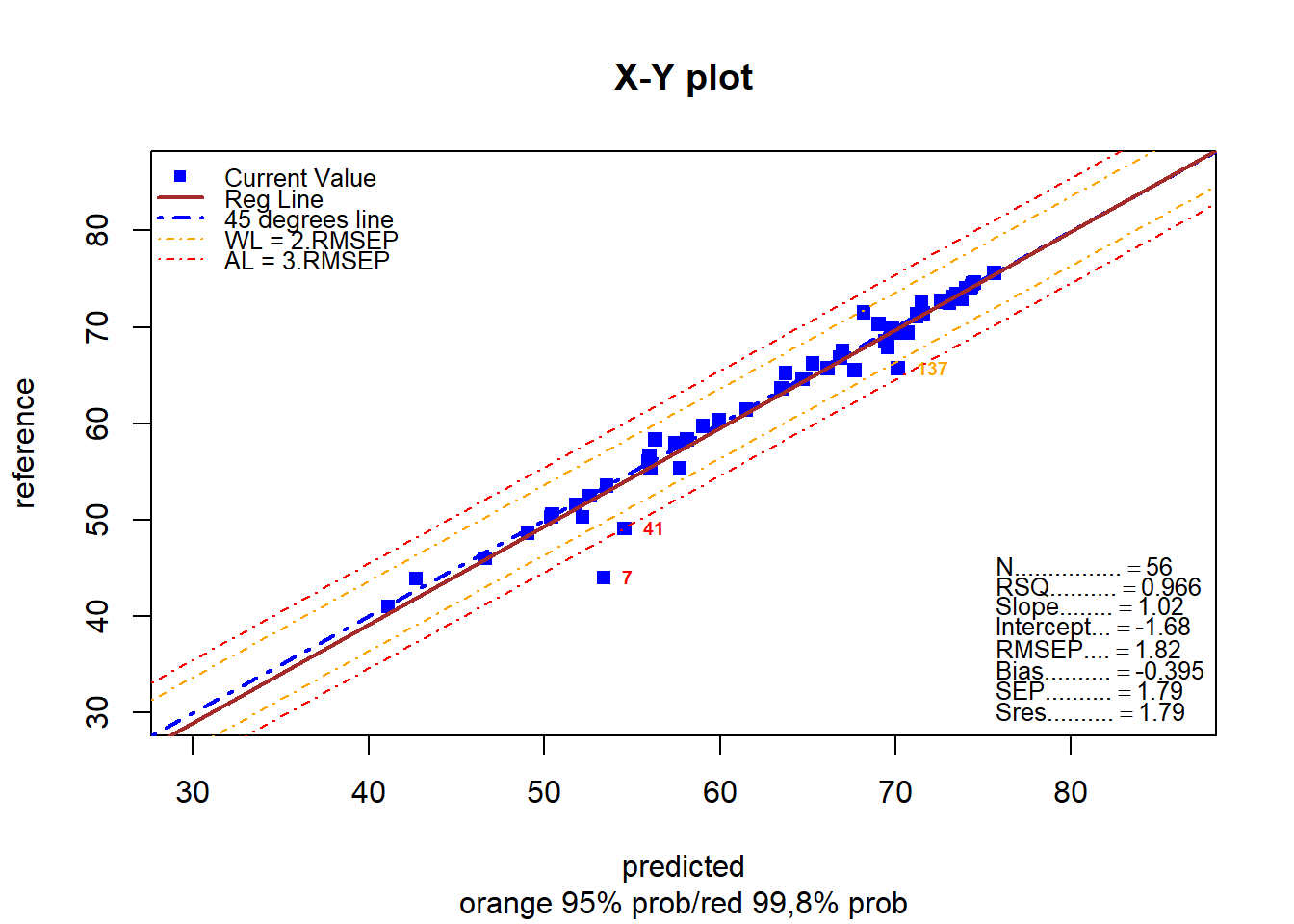
$ResWarning
   index  id  ref     pred       res res.corr1 res.corr2  Q   Color
38    38 137 65.7 70.14363 -4.443631     -4.05     -4.18 Q1 #00CC66

$ResWarningList
[1] 38

$ResAction
   index id  ref     pred       res res.corr1 res.corr2          Q   Color
3      3  7 44.0 53.40620 -9.406203     -9.01     -8.80 Q1 to MIN  #0000FF
17    17 41 49.1 54.57022 -5.470218     -5.07     -4.89 Q1 to MIN  #0000FF

$ResActionList
[1]  3 17
As we can see the statistics are quite good for all the parameters (specially for fat and moisture), and show us that this algorithm must be considered when developing NIR models.