Near Infrared Transmitance Tutorial (part 4)

Organizing data

Let´s see what we have in the workspace from the previous posts:

load("C:/BLOG/Workspaces/NIT Tutorial/NIT_ws3.RData")
ls()

[1] "absorp"           "cor_rawspec"      "cor_rawspec_fat"  "cor_rawspec_moi" 
[5] "cor_rawspec_prot" "endpoints"        "meats"            "meats_longer"    
[9] "tecator"         

We can remove some objects we don´t need

rm("cor_rawspec_fat", "cor_rawspec_moi", "cor_rawspec_prot")

Now we load the libraries we will use:

library(tidyverse)

Scatter correction math-treatments

The idea now is to apply some math treatments to the raw spectra and check which one improves the correlation with the parameters of interest. Normally there are some common scatter removal algorithms that I use:

• Standard Normal Variate (SNV)

• Detrend (linear or quadratic)

• SNV + Detrend (linear or quadratic)

• Multiple Scatter Correction

There are some packages in R which have these math treatment with this name or a similar one, or we can create functions to apply these algorithms to the spectra matrix.

Standard Normal Variate (SNV)

Let´s start using SNV, where we center every spectrum (subtracting the mean) and scale it (dividing by the standard deviation):

#The algorithm is applied to the columns, so we transpose the matrix
absorp_snv <- scale(t(absorp), center = TRUE, scale = TRUE)
#Let´s convert the corrected matrix as usual
absorp_snv <- t(absorp_snv)

matplot(colnames(absorp_snv), t(absorp_snv), type = "l", xlab = "Wavelength (nm)", ylab = "Absorbance", main = "SNV Meat Spectra")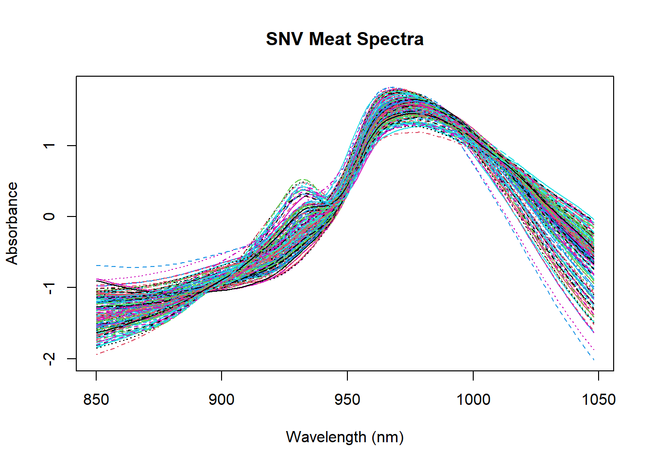

Figure 1: Meat spectra treated with SNV.

We can add the matrix treated with the SNV math treatment to the tecator dataframe

tecator$snv_spec <- absorp_snv

Correlation between outcomes and predictors (with SNV)

Now we can see if the correlation is improved

cor_snvspec_moi <- cor(tecator$Moisture, tecator$snv_spec)
cor_snvspec_fat <- cor(tecator$Fat, tecator$snv_spec)
cor_snvspec_prot <- cor(tecator$Protein, tecator$snv_spec)

cor_snvspec <- as.data.frame(rbind(cor_snvspec_moi, cor_snvspec_fat, cor_snvspec_prot))

cor_snvspec <- cor_snvspec %>% 
  mutate(Parameter = as.factor(c("Moisture", "Fat", "Protein")))

cor_snvspec %>% 
  pivot_longer(cols = c(1:100), names_to = "Wavelength", values_to = "Correlation") %>% 
  mutate(Wavelength = as.integer(Wavelength)) %>% 
  ggplot(aes(x = Wavelength, y = Correlation, group = Parameter, col = Parameter)) +
  geom_line()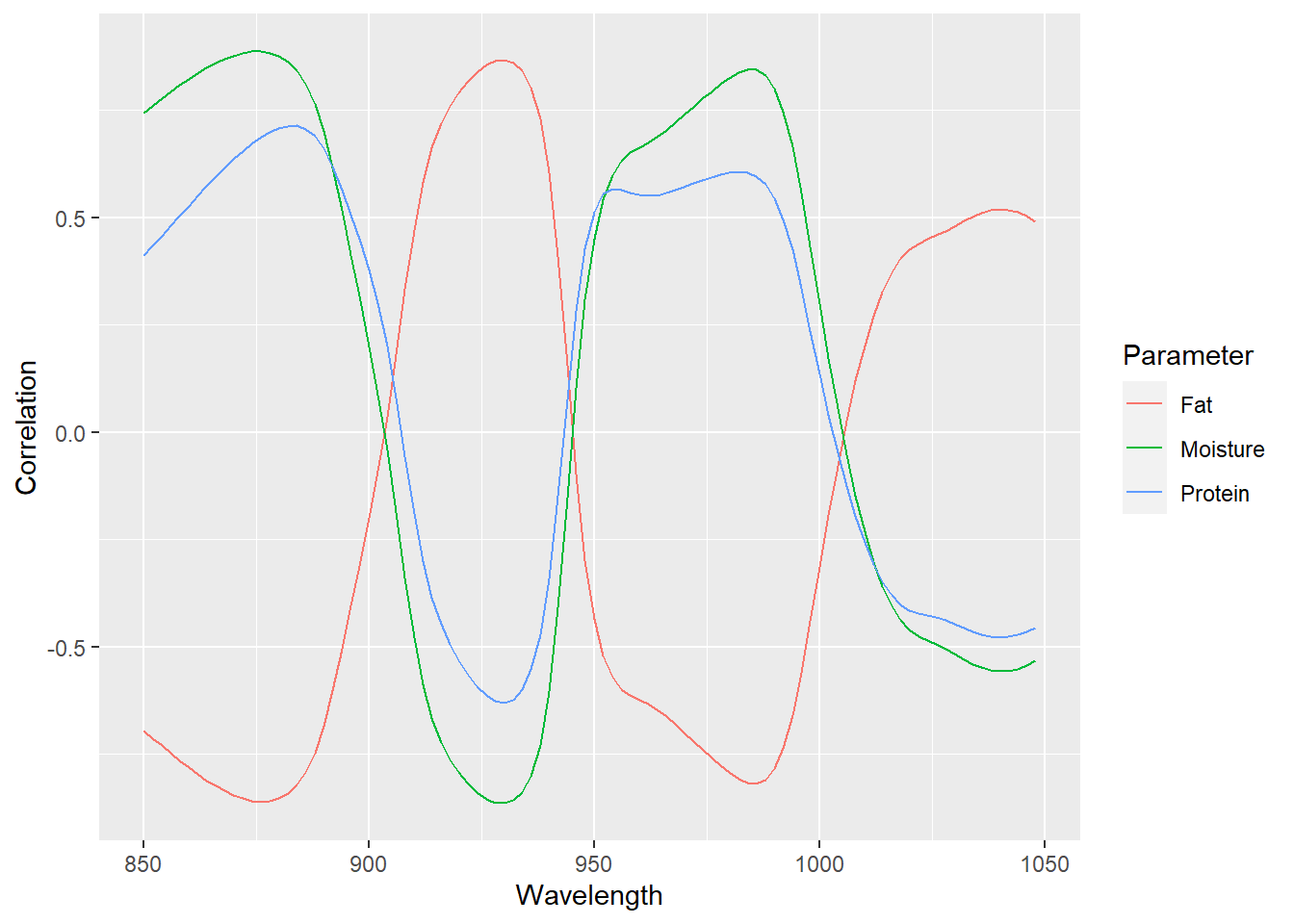

Figure 2: Correlation SNV signal with the parametes.

Now, apart from the better correlation we can see an improvement in the definition of the correlations (positives and negatives), and the correlation spectra confirm what we have seen in the correlation between the parameters.

As always save the workspace for future use:

save.image("C:/BLOG/Workspaces/NIT Tutorial/NIT_ws4.RData")